Unified Calculus Formula Book (Calculus I, II, & III)

Engineering Mathematics Reference Guide (MATH 181 • MATH 182 • MATH 283)

This unified reference document provides a clean, formula-only reference manual for students across single-variable and multivariable engineering calculus.

1. Pre-Calculus, Algebra, & Geometry

1.1 Algebra & Factoring Formulas

• Difference of Squares: $a^2 - b^2 = (a - b)(a + b)$
• Difference of Cubes: $a^3 - b^3 = (a - b)(a^2 + ab + b^2)$
• Sum of Cubes: $a^3 + b^3 = (a + b)(a^2 - ab + b^2)$
• Binomial Expansions:
  • $(a + b)^2 = a^2 + 2ab + b^2$
  • $(a - b)^2 = a^2 - 2ab + b^2$
  • $(a + b)^3 = a^3 + 3a^2b + 3ab^2 + b^3$
  • $(a - b)^3 = a^3 - 3a^2b + 3ab^2 - b^3$
• Quadratic Formula: For $ax^2 + bx + c = 0$, $x = \frac{-b \pm \sqrt{b^2 - 4ac}}{2a}$

1.2 Exponents & Logarithms

• $a^{x+y} = a^x a^y, \quad a^{x-y} = \frac{a^x}{a^y}, \quad (a^x)^y = a^{xy}, \quad a^{-x} = \frac{1}{a^x}, \quad a^{1/n} = \sqrt[n]{a}$
• $\ln(xy) = \ln x + \ln y, \quad \ln\left(\frac{x}{y}\right) = \ln x - \ln y, \quad \ln(x^r) = r\ln x$
• $\ln(1) = 0, \quad \ln(e) = 1, \quad e^{\ln x} = x, \quad \ln(e^x) = x$
• Change of Base: $\log_a x = \frac{\ln x}{\ln a} = \frac{\log_{10} x}{\log_{10} a}$

1.3 Geometric Formulas

1.4 Trigonometric Functions & The Unit Circle

Fundamental Identities

• Reciprocal & Quotient:
  $$\tan\theta = \frac{\sin\theta}{\cos\theta}, \quad \cot\theta = \frac{\cos\theta}{\sin\theta}, \quad \sec\theta = \frac{1}{\cos\theta}, \quad \csc\theta = \frac{1}{\sin\theta}$$
• Pythagorean Identities:
  $$\sin^2\theta + \cos^2\theta = 1, \quad 1 + \tan^2\theta = \sec^2\theta, \quad 1 + \cot^2\theta = \csc^2\theta$$
• Even/Odd Symmetries:
  $$\sin(-\theta) = -\sin\theta, \quad \cos(-\theta) = \cos\theta, \quad \tan(-\theta) = -\tan\theta$$

Sum, Difference, & Angle Formulas

• Sum & Difference:
  $$\sin(A \pm B) = \sin A \cos B \pm \cos A \sin B$$
  $$\cos(A \pm B) = \cos A \cos B \mp \sin A \sin B$$
  $$\tan(A \pm B) = \frac{\tan A \pm \tan B}{1 \mp \tan A \tan B}$$
• Double-Angle Identities:
  $$\sin(2\theta) = 2\sin\theta\cos\theta$$
  $$\cos(2\theta) = \cos^2\theta - \sin^2\theta = 2\cos^2\theta - 1 = 1 - 2\sin^2\theta$$
  $$\tan(2\theta) = \frac{2\tan\theta}{1 - \tan^2\theta}$$
• Half-Angle / Power-Reduction Identities:
  $$\sin^2\theta = \frac{1 - \cos(2\theta)}{2}, \quad \cos^2\theta = \frac{1 + \cos(2\theta)}{2}, \quad \tan^2\theta = \frac{1 - \cos(2\theta)}{1 + \cos(2\theta)}$$
• Product-to-Sum Identities:
  $$\sin A \cos B = \frac{1}{2}[\sin(A + B) + \sin(A - B)]$$
  $$\cos A \cos B = \frac{1}{2}[\cos(A + B) + \cos(A - B)]$$
  $$\sin A \sin B = \frac{1}{2}[\cos(A - B) - \cos(A + B)]$$

2. Calculus I (Single-Variable Differential Calculus)

2.1 Limits & Continuity

• Definition of Derivative: $f'(x) = \lim_{h \to 0} \frac{f(x+h) - f(x)}{h} = \lim_{z \to x}\frac{f(z) - f(x)}{z - x}$
• Continuity at $x = a$: $f(a)$ is defined, $\lim_{x \to a} f(x)$ exists, and $\lim_{x \to a} f(x) = f(a)$.
• Special Limits:
  $$\lim_{\theta \to 0} \frac{\sin\theta}{\theta} = 1, \quad \lim_{\theta \to 0} \frac{1 - \cos\theta}{\theta} = 0, \quad \lim_{n \to \infty}\left(1 + \frac{1}{n}\right)^n = e$$
• L'Hôpital's Rule: For indeterminate forms $\left[\frac{0}{0}\right]$ or $\left[\frac{\pm\infty}{\pm\infty}\right]$, $\lim_{x \to a}\frac{f(x)}{g(x)} = \lim_{x \to a}\frac{f'(x)}{g'(x)}$

2.2 Differentiation Rules

• Constant Rule: $\frac{d}{dx}[c] = 0$
• Power Rule: $\frac{d}{dx}[x^n] = n x^{n-1}$
• Constant Multiple: $\frac{d}{dx}[c f(x)] = c f'(x)$
• Sum & Difference: $\frac{d}{dx}[f(x) \pm g(x)] = f'(x) \pm g'(x)$
• Product Rule: $\frac{d}{dx}[f(x) g(x)] = f'(x)g(x) + f(x)g'(x)$
• Quotient Rule: $\frac{d}{dx}\left[\frac{f(x)}{g(x)}\right] = \frac{f'(x)g(x) - f(x)g'(x)}{[g(x)]^2}$
• Chain Rule: $\frac{d}{dx}[f(g(x))] = f'(g(x)) g'(x)$

2.3 Table of Derivatives

2.4 Applications of Derivatives

• Linearization / Tangent Line: $L(x) = f(a) + f'(a)(x - a)$
• Newton's Method: $x_{n+1} = x_n - \frac{f(x_n)}{f'(x_n)}$
• Mean Value Theorem: If $f$ is continuous on $[a,b]$ and differentiable on $(a,b)$, then there exists $c \in (a,b)$ such that $f'(c) = \frac{f(b) - f(a)}{b - a}$.
• Extreme Value Analysis:
  • Critical points occur where $f'(c) = 0$ or $f'(c)$ is undefined.
  • Second Derivative Test: If $f'(c) = 0$:
    • $f''(c) > 0 \implies$ Local Minimum (concave up)
    • $f''(c) < 0 \implies$ Local Maximum (concave down)
    • $f''(c) = 0 \implies$ Inconclusive

3. Calculus II (Integral Calculus, Techniques, Series, & Parametrics)

3.1 Fundamental Theorems & Basic Integrals

• FTC Part 1: $\frac{d}{dx}\left[ \int_{a}^{x} f(t)\,dt \right] = f(x) \quad \text{and} \quad \frac{d}{dx}\left[ \int_{g(x)}^{h(x)} f(t)\,dt \right] = f(h(x))h'(x) - f(g(x))g'(x)$
• FTC Part 2 (Evaluation): $\int_{a}^{b} f(x)\,dx = F(b) - F(a) = [F(x)]_a^b$, where $F'(x) = f(x)$.
• Net Change Theorem: $\int_a^b f'(t)\,dt = f(b) - f(a)$
• Average Value: $f_{\text{avg}} = \frac{1}{b - a}\int_a^b f(x)\,dx$

3.2 Table of Indefinite Integrals

3.3 Integration Techniques

• Substitution Method ($u$-sub): $\int f(g(x))g'(x)\,dx = \int f(u)\,du$
• Integration by Parts: $\int u\,dv = uv - \int v\,du$
  • Definite: $\int_a^b u\,dv = [uv]_a^b - \int_a^b v\,du$
• Trigonometric Substitution:
  • For $\sqrt{a^2 - x^2}$: Substitute $x = a\sin\theta$, $dx = a\cos\theta\,d\theta$, identity: $\sqrt{a^2 - x^2} = a\cos\theta$
  • For $\sqrt{a^2 + x^2}$: Substitute $x = a\tan\theta$, $dx = a\sec^2\theta\,d\theta$, identity: $\sqrt{a^2 + x^2} = a\sec\theta$
  • For $\sqrt{x^2 - a^2}$: Substitute $x = a\sec\theta$, $dx = a\sec\theta\tan\theta\,d\theta$, identity: $\sqrt{x^2 - a^2} = a\tan\theta$
• Improper $p$-Integrals: $\int_{1}^{\infty} \frac{1}{x^p}\,dx$ converges if and only if $p > 1$.

3.4 Applications of Integrals

• Area Between Curves: $A = \int_a^b |f(x) - g(x)|\,dx$
• Volumes of Solids of Revolution:
  • Disk Method (Axis $\parallel x$-axis): $V = \pi \int_a^b [R(x)]^2\,dx$
  • Washer Method: $V = \pi \int_a^b \left( [R(x)]^2 - [r(x)]^2 \right)\,dx$
  • Cylindrical Shells: $V = 2\pi \int_a^b (\text{radius})(\text{height})\,dx = 2\pi \int_a^b x [f(x) - g(x)]\,dx$
• Arc Length (2D):
  • Cartesian: $s = \int_a^b \sqrt{1 + [f'(x)]^2}\,dx$
  • Parametric: $s = \int_\alpha^\beta \sqrt{[x'(t)]^2 + [y'(t)]^2}\,dt$
  • Polar: $s = \int_\alpha^\beta \sqrt{r^2 + \left(\frac{dr}{d\theta}\right)^2}\,d\theta$
• Surface Area of Revolution: $S = 2\pi \int r\,ds$
• Physical Applications:
  • Work: $W = \int_a^b F(x)\,dx$; Hooke's Law: $F(x) = kx \implies W = \frac{1}{2}k x^2$
  • Hydrostatic Force: $F = \int_a^b \rho g (d - y) w(y)\,dy$
  • Centroid Coordinates: $\bar{x} = \frac{1}{A}\int_a^b x[f(x)-g(x)]\,dx, \quad \bar{y} = \frac{1}{2A}\int_a^b \left([f(x)]^2 - [g(x)]^2\right)\,dx$

3.5 Infinite Sequences & Series

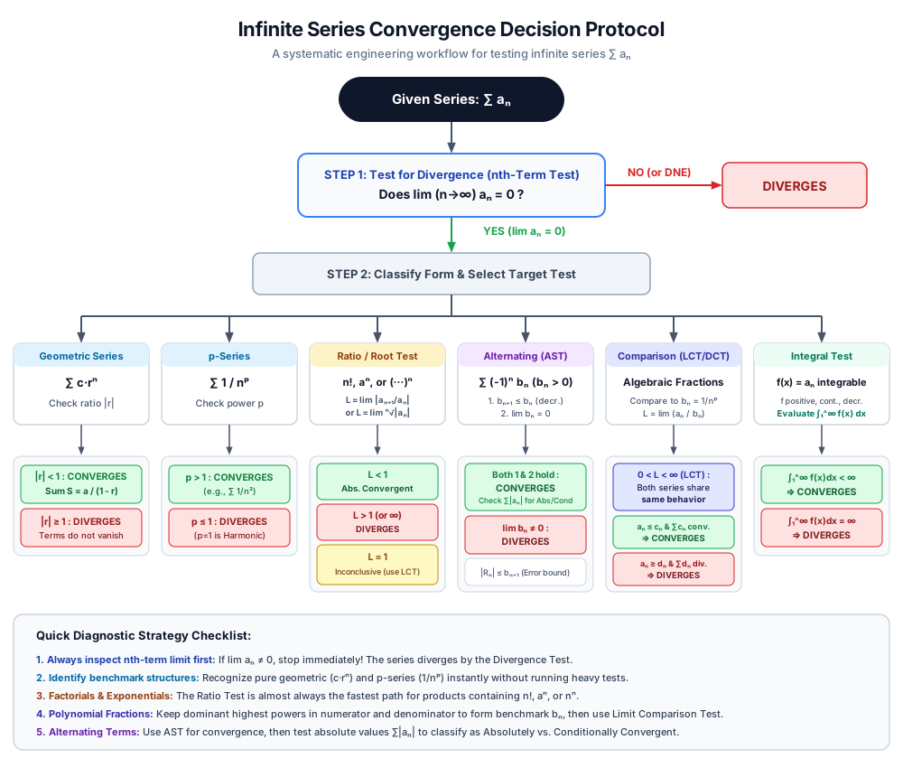
Convergence Tests Flowchart

Power Series, Taylor & Maclaurin Expansions

• Taylor Series about $x = a$:
  $$f(x) = \sum_{n=0}^{\infty} \frac{f^{(n)}(a)}{n!}(x - a)^n = f(a) + f'(a)(x - a) + \frac{f''(a)}{2!}(x - a)^2 + \cdots$$
• Maclaurin Series ($a = 0$): $f(x) = \sum_{n=0}^{\infty} \frac{f^{(n)}(0)}{n!}x^n$
• Standard Maclaurin Series:
  $$\frac{1}{1 - x} = \sum_{n=0}^{\infty} x^n = 1 + x + x^2 + x^3 + \cdots \quad (|x| < 1)$$
  $$e^x = \sum_{n=0}^{\infty} \frac{x^n}{n!} = 1 + x + \frac{x^2}{2!} + \frac{x^3}{3!} + \cdots \quad (-\infty < x < \infty)$$
  $$\sin x = \sum_{n=0}^{\infty} (-1)^n \frac{x^{2n+1}}{(2n+1)!} = x - \frac{x^3}{3!} + \frac{x^5}{5!} - \cdots \quad (-\infty < x < \infty)$$
  $$\cos x = \sum_{n=0}^{\infty} (-1)^n \frac{x^{2n}}{(2n)!} = 1 - \frac{x^2}{2!} + \frac{x^4}{4!} - \cdots \quad (-\infty < x < \infty)$$
  $$\ln(1 + x) = \sum_{n=1}^{\infty} (-1)^{n-1} \frac{x^n}{n} = x - \frac{x^2}{2} + \frac{x^3}{3} - \cdots \quad (-1 < x \le 1)$$
  $$\arctan x = \sum_{n=0}^{\infty} (-1)^n \frac{x^{2n+1}}{2n+1} = x - \frac{x^3}{3} + \frac{x^5}{5} - \cdots \quad (-1 \le x \le 1)$$
  $$(1 + x)^k = 1 + kx + \frac{k(k-1)}{2!}x^2 + \frac{k(k-1)(k-2)}{3!}x^3 + \cdots \quad (|x| < 1)$$

4. Calculus III (Multivariable & Vector Calculus for Engineers)

4.1 3D Coordinate Geometry & Vectors

• 3D Distance Formula: $d = \sqrt{(x_2 - x_1)^2 + (y_2 - y_1)^2 + (z_2 - z_1)^2}$
• Sphere Equation: $(x - x_0)^2 + (y - y_0)^2 + (z - z_0)^2 = R^2$
• Magnitude & Unit Vector:
  $$\|\vec{v}\| = \sqrt{v_1^2 + v_2^2 + v_3^2}, \quad \hat{u} = \frac{\vec{v}}{\|\vec{v}\|}$$
• Dot Product:
  $$\vec{u} \cdot \vec{v} = u_1 v_1 + u_2 v_2 + u_3 v_3 = \|\vec{u}\|\|\vec{v}\|\cos\theta$$
  • Orthogonality Condition: $\vec{u} \perp \vec{v} \iff \vec{u} \cdot \vec{v} = 0$
  • Angle: $\cos\theta = \frac{\vec{u} \cdot \vec{v}}{\|\vec{u}\|\|\vec{v}\|}$
• Scalar & Vector Projections:
  $$\text{scal}_{\vec{u}}\vec{v} = \frac{\vec{u} \cdot \vec{v}}{\|\vec{u}\|}$$
  $$\text{proj}_{\vec{u}}\vec{v} = \left(\frac{\vec{u} \cdot \vec{v}}{\|\vec{u}\|^2}\right)\vec{u} = \left(\frac{\vec{u} \cdot \vec{v}}{\vec{u} \cdot \vec{u}}\right)\vec{u}$$
  $$\text{orth}_{\vec{u}}\vec{v} = \vec{v} - \text{proj}_{\vec{u}}\vec{v}$$
• Cross Product:
  $$\vec{u} \times \vec{v} = \begin{vmatrix} \hat{i} & \hat{j} & \hat{k} \\ u_1 & u_2 & u_3 \\ v_1 & v_2 & v_3 \end{vmatrix} = \langle u_2 v_3 - u_3 v_2, \; u_3 v_1 - u_1 v_3, \; u_1 v_2 - u_2 v_1 \rangle$$
  • Magnitude: $\|\vec{u} \times \vec{v}\| = \|\vec{u}\|\|\vec{v}\|\sin\theta$
  • Parallel Condition: $\vec{u} \parallel \vec{v} \iff \vec{u} \times \vec{v} = \vec{0}$
  • Geometric Area of Parallelogram $= \|\vec{u} \times \vec{v}\|$; Area of Triangle $= \frac{1}{2}\|\vec{u} \times \vec{v}\|$
  • Torque: $\vec{\tau} = \vec{r} \times \vec{F}$
• Triple Scalar Product & Volume:
  $$\vec{u} \cdot (\vec{v} \times \vec{w}) = \begin{vmatrix} u_1 & u_2 & u_3 \\ v_1 & v_2 & v_3 \\ w_1 & w_2 & w_3 \end{vmatrix}$$
  • Parallelepiped Volume: $V = |\vec{u} \cdot (\vec{v} \times \vec{w})|$
  • Coplanarity Condition: $\vec{u}, \vec{v}, \vec{w}$ are coplanar $\iff \vec{u} \cdot (\vec{v} \times \vec{w}) = 0$

4.2 Lines & Distances in 3D Space

• Equations of a Line through $P_0(x_0, y_0, z_0)$ with Direction $\vec{v} = \langle a, b, c \rangle$:
  • Vector Equation: $\vec{r}(t) = \vec{r}_0 + t\vec{v} = \langle x_0 + at, y_0 + bt, z_0 + ct \rangle$
  • Parametric Equations: $x = x_0 + at, \quad y = y_0 + bt, \quad z = z_0 + ct$
  • Symmetric Equations: $\frac{x - x_0}{a} = \frac{y - y_0}{b} = \frac{z - z_0}{c} \quad (abc \ne 0)$
• Shortest Distance from Point $M$ to Line $L$ (Point $P \in L$, Direction $\vec{v}$):
  $$d = \frac{\|\vec{PM} \times \vec{v}\|}{\|\vec{v}\|}$$
• Classification of Two 3D Lines $L_1(\vec{r}_1(t) = \vec{r}_{01} + t\vec{v}_1)$ and $L_2(\vec{r}_2(s) = \vec{r}_{02} + s\vec{v}_2)$:
  1. Parallel: $\vec{v}_1 = k\vec{v}_2$. (Coincident if points on $L_1$ satisfy $L_2$, otherwise Distinct Parallel).
  2. Intersecting: $\vec{v}_1 \ne k\vec{v}_2$ and the linear system $\vec{r}_1(t) = \vec{r}_2(s)$ has a consistent unique solution $(t^*, s^*)$.
  3. Skew: $\vec{v}_1 \ne k\vec{v}_2$ and the linear system $\vec{r}_1(t) = \vec{r}_2(s)$ is inconsistent (lines are non-parallel and non-intersecting).

4.3 Vector-Valued Functions, Curves, & Kinematics

• Kinematic Hierarchy:
  • Position: $\vec{r}(t) = \langle x(t), y(t), z(t) \rangle$
  • Velocity: $\vec{v}(t) = \vec{r}'(t) = \langle x'(t), y'(t), z'(t) \rangle$
  • Acceleration: $\vec{a}(t) = \vec{r}''(t) = \vec{v}'(t) = \langle x''(t), y''(t), z''(t) \rangle$
  • Scalar Speed: $v(t) = \|\vec{v}(t)\| = \sqrt{(x')^2 + (y')^2 + (z')^2}$
• Arc Length & Intrinsic Parametrization:
  • Arc Length Integral: $s = \int_{a}^{b} \|\vec{r}'(t)\|\,dt$
  • Accumulated Arc Length Function: $s(t) = \int_{a}^{t} \|\vec{r}'(u)\|\,du \implies \frac{ds}{dt} = \|\vec{r}'(t)\|$
  • Unit Speed Property under $\vec{r}(s)$: $\|\vec{r}'(s)\| = 1$
• TNB Frame & Curvature:
  • Unit Tangent Vector: $\hat{T}(t) = \frac{\vec{r}'(t)}{\|\vec{r}'(t)\|}$
  • Principal Unit Normal Vector: $\hat{N}(t) = \frac{\hat{T}'(t)}{\|\hat{T}'(t)\|}$
  • Binormal Vector: $\hat{B}(t) = \hat{T}(t) \times \hat{N}(t)$
  • Curvature Formulas:
    $$\kappa = \frac{\|\hat{T}'(t)\|}{\|\vec{r}'(t)\|} = \frac{\|\vec{r}'(t) \times \vec{r}''(t)\|}{\|\vec{r}'(t)\|^3} = \frac{\|\vec{v} \times \vec{a}\|}{v^3}$$
    For planar curve $y = f(x)$: $\kappa(x) = \frac{|f''(x)|}{[1 + (f'(x))^2]^{3/2}}$
  • Radius of Curvature & Osculating Circle: $\rho = \frac{1}{\kappa}$
• Tangential & Normal Acceleration Decomposition:
  $$\vec{a}(t) = a_T \hat{T}(t) + a_N \hat{N}(t)$$
  $$a_T = \frac{d}{dt}\|\vec{v}\| = \frac{\vec{v} \cdot \vec{a}}{\|\vec{v}\|}$$
  $$a_N = \kappa \|\vec{v}\|^2 = \frac{\|\vec{v} \times \vec{a}\|}{\|\vec{v}\|} = \sqrt{\|\vec{a}\|^2 - a_T^2} \quad (a_N \ge 0)$$

4.4 Multivariable Differential Calculus

• Partial Derivatives: $f_x = \frac{\partial f}{\partial x} = \lim_{h \to 0}\frac{f(x+h, y) - f(x,y)}{h}, \quad f_y = \frac{\partial f}{\partial y} = \lim_{h \to 0}\frac{f(x, y+h) - f(x,y)}{h}$
• Clairaut's Theorem: If $f_{xy}$ and $f_{yx}$ are continuous, then $f_{xy} = f_{yx}$.
• Tangent Plane to $z = f(x,y)$ at $(x_0, y_0, z_0)$:
  $$z - z_0 = f_x(x_0, y_0)(x - x_0) + f_y(x_0, y_0)(y - y_0)$$
• Linear Approximation & Total Differential:
  $$L(x,y) = f(x_0, y_0) + f_x(x_0, y_0)(x - x_0) + f_y(x_0, y_0)(y - y_0)$$
  $$dz = \frac{\partial z}{\partial x}dx + \frac{\partial z}{\partial y}dy$$
• Multivariable Chain Rule:
  • If $z = f(x,y)$ where $x = g(t), y = h(t)$: $\frac{dz}{dt} = \frac{\partial z}{\partial x}\frac{dx}{dt} + \frac{\partial z}{\partial y}\frac{dy}{dt}$
  • If $z = f(x,y)$ where $x = g(u,v), y = h(u,v)$: $\frac{\partial z}{\partial u} = \frac{\partial z}{\partial x}\frac{\partial x}{\partial u} + \frac{\partial z}{\partial y}\frac{\partial y}{\partial u}$
• Gradient Vector & Directional Derivative:
  $$\nabla f = \left\langle \frac{\partial f}{\partial x}, \frac{\partial f}{\partial y}, \frac{\partial f}{\partial z} \right\rangle$$
  $$D_{\hat{u}}f = \nabla f \cdot \hat{u} \quad (\|\hat{u}\| = 1)$$
  • Maximum rate of increase is $\|\nabla f\|$, occurring in the direction of $\hat{u} = \frac{\nabla f}{\|\nabla f\|}$.
  • Tangent plane to level surface $F(x,y,z) = C$ at $P_0$: $\nabla F(P_0) \cdot \langle x - x_0, y - y_0, z - z_0 \rangle = 0$.
• Critical Points & Second Derivative Test:
  • Critical points occur where $\nabla f(x_0, y_0) = \vec{0}$ or is undefined.
  • Discriminant: $D = f_{xx}f_{yy} - (f_{xy})^2$
    • $D > 0 \text{ and } f_{xx} > 0 \implies$ Local Minimum
    • $D > 0 \text{ and } f_{xx} < 0 \implies$ Local Maximum
    • $D < 0 \implies$ Saddle Point
    • $D = 0 \implies$ Inconclusive
• Lagrange Multipliers: To optimize $f(x,y,z)$ subject to constraint $g(x,y,z) = k$:
  $$\nabla f = \lambda \nabla g \quad \text{and} \quad g(x,y,z) = k$$

4.5 Multiple Integrals & Coordinate Transformations

• Double Integrals:
  • Rectangular: $\iint_R f(x,y)\,dA = \int_a^b \int_c^d f(x,y)\,dy\,dx$
  • Polar Coordinates ($x = r\cos\theta, y = r\sin\theta, x^2 + y^2 = r^2$):
    $$\iint_R f(x,y)\,dA = \iint_R f(r\cos\theta, r\sin\theta)\,r\,dr\,d\theta$$
• Triple Integrals:
  • Rectangular: $dV = dx\,dy\,dz$
  • Cylindrical ($x = r\cos\theta, y = r\sin\theta, z = z$):
    $$dV = r\,dr\,d\theta\,dz$$
  • Spherical ($x = \rho\sin\phi\cos\theta, y = \rho\sin\phi\sin\theta, z = \rho\cos\phi, x^2 + y^2 + z^2 = \rho^2$):
    $$dV = \rho^2 \sin\phi\,d\rho\,d\phi\,d\theta \quad (0 \le \phi \le \pi, \; 0 \le \theta \le 2\pi)$$
• Jacobian Transformation (2D & 3D):
  $$J(u,v) = \frac{\partial(x,y)}{\partial(u,v)} = \begin{vmatrix} \frac{\partial x}{\partial u} & \frac{\partial x}{\partial v} \\ \frac{\partial y}{\partial u} & \frac{\partial y}{\partial v} \end{vmatrix} \implies dA = |J(u,v)|\,du\,dv$$
• Physical Applications of Multiple Integrals:
  • Mass: $M = \iint_D \rho(x,y)\,dA \quad \text{or} \quad M = \iiint_E \rho(x,y,z)\,dV$
  • Center of Mass: $\bar{x} = \frac{1}{M}\iint_D x\rho\,dA, \quad \bar{y} = \frac{1}{M}\iint_D y\rho\,dA$