🌱 Tony's Memex Tony's Intertwingled Memex
Digital Garden | OER Curriculum
Home / Digital Garden / Unified Calculus Formula Book (Calculus I, II, & III)

Unified Calculus Formula Book (Calculus I, II, & III)

Engineering Mathematics Reference Guide (MATH 181 • MATH 182 • MATH 283)

This unified reference document provides a clean, formula-only reference manual for students across single-variable and multivariable engineering calculus.


1. Pre-Calculus, Algebra, & Geometry

1.1 Algebra & Factoring Formulas

  • Difference of Squares: a2−b2=(a−b)(a+b)a^2 - b^2 = (a - b)(a + b)
  • Difference of Cubes: a3−b3=(a−b)(a2+ab+b2)a^3 - b^3 = (a - b)(a^2 + ab + b^2)
  • Sum of Cubes: a3+b3=(a+b)(a2−ab+b2)a^3 + b^3 = (a + b)(a^2 - ab + b^2)
  • Binomial Expansions:
    • (a+b)2=a2+2ab+b2(a + b)^2 = a^2 + 2ab + b^2
    • (a−b)2=a2−2ab+b2(a - b)^2 = a^2 - 2ab + b^2
    • (a+b)3=a3+3a2b+3ab2+b3(a + b)^3 = a^3 + 3a^2b + 3ab^2 + b^3
    • (a−b)3=a3−3a2b+3ab2−b3(a - b)^3 = a^3 - 3a^2b + 3ab^2 - b^3
  • Quadratic Formula: For ax2+bx+c=0ax^2 + bx + c = 0, x=−b±b2−4ac2ax = \frac{-b \pm \sqrt{b^2 - 4ac}}{2a}

1.2 Exponents & Logarithms

  • ax+y=axay,ax−y=axay,(ax)y=axy,a−x=1ax,a1/n=ana^{x+y} = a^x a^y, \quad a^{x-y} = \frac{a^x}{a^y}, \quad (a^x)^y = a^{xy}, \quad a^{-x} = \frac{1}{a^x}, \quad a^{1/n} = \sqrt[n]{a}
  • ln⁡(xy)=ln⁡x+ln⁡y,ln⁡(xy)=ln⁡x−ln⁡y,ln⁡(xr)=rln⁡x\ln(xy) = \ln x + \ln y, \quad \ln\left(\frac{x}{y}\right) = \ln x - \ln y, \quad \ln(x^r) = r\ln x
  • ln⁡(1)=0,ln⁡(e)=1,eln⁡x=x,ln⁡(ex)=x\ln(1) = 0, \quad \ln(e) = 1, \quad e^{\ln x} = x, \quad \ln(e^x) = x
  • Change of Base: log⁡ax=ln⁡xln⁡a=log⁡10xlog⁡10a\log_a x = \frac{\ln x}{\ln a} = \frac{\log_{10} x}{\log_{10} a}

1.3 Geometric Formulas

Shape / Solid Perimeter / Surface Area Area / Volume
Circle (Radius rr) C=2πr=πdC = 2\pi r = \pi d A=πr2A = \pi r^2
Triangle (Base bb, Height hh) P=a+b+cP = a + b + c A=12bhA = \frac{1}{2}bh
Trapezoid (Bases a,ba, b, Height hh) P=a+b+c+dP = a + b + c + d A=a+b2hA = \frac{a + b}{2}h
Sphere (Radius rr) A=4πr2A = 4\pi r^2 V=43πr3V = \frac{4}{3}\pi r^3
Right Circular Cylinder (r,hr, h) A=2πr2+2πrhA = 2\pi r^2 + 2\pi rh (total) V=πr2hV = \pi r^2 h
Right Circular Cone (r,hr, h) A=πr2+πrr2+h2A = \pi r^2 + \pi r\sqrt{r^2 + h^2} V=13πr2hV = \frac{1}{3}\pi r^2 h
Rectangular Box (l,w,hl, w, h) A=2(lw+lh+wh)A = 2(lw + lh + wh) V=lwhV = lwh

1.4 Trigonometric Functions & The Unit Circle

Unit Circle Reference

Fundamental Identities

  • Reciprocal & Quotient:
    tan⁡θ=sin⁡θcos⁡θ,cot⁡θ=cos⁡θsin⁡θ,sec⁡θ=1cos⁡θ,csc⁡θ=1sin⁡θ\tan\theta = \frac{\sin\theta}{\cos\theta}, \quad \cot\theta = \frac{\cos\theta}{\sin\theta}, \quad \sec\theta = \frac{1}{\cos\theta}, \quad \csc\theta = \frac{1}{\sin\theta}
  • Pythagorean Identities:
    sin⁡2θ+cos⁡2θ=1,1+tan⁡2θ=sec⁡2θ,1+cot⁡2θ=csc⁡2θ\sin^2\theta + \cos^2\theta = 1, \quad 1 + \tan^2\theta = \sec^2\theta, \quad 1 + \cot^2\theta = \csc^2\theta
  • Even/Odd Symmetries:
    sin⁡(−θ)=−sin⁡θ,cos⁡(−θ)=cos⁡θ,tan⁡(−θ)=−tan⁡θ\sin(-\theta) = -\sin\theta, \quad \cos(-\theta) = \cos\theta, \quad \tan(-\theta) = -\tan\theta

Sum, Difference, & Angle Formulas

  • Sum & Difference:
    sin⁡(A±B)=sin⁡Acos⁡B±cos⁡Asin⁡B\sin(A \pm B) = \sin A \cos B \pm \cos A \sin B
    cos⁡(A±B)=cos⁡Acos⁡B∓sin⁡Asin⁡B\cos(A \pm B) = \cos A \cos B \mp \sin A \sin B
    tan⁡(A±B)=tan⁡A±tan⁡B1∓tan⁡Atan⁡B\tan(A \pm B) = \frac{\tan A \pm \tan B}{1 \mp \tan A \tan B}
  • Double-Angle Identities:
    sin⁡(2θ)=2sin⁡θcos⁡θ\sin(2\theta) = 2\sin\theta\cos\theta
    cos⁡(2θ)=cos⁡2θ−sin⁡2θ=2cos⁡2θ−1=1−2sin⁡2θ\cos(2\theta) = \cos^2\theta - \sin^2\theta = 2\cos^2\theta - 1 = 1 - 2\sin^2\theta
    tan⁡(2θ)=2tan⁡θ1−tan⁡2θ\tan(2\theta) = \frac{2\tan\theta}{1 - \tan^2\theta}
  • Half-Angle / Power-Reduction Identities:
    sin⁡2θ=1−cos⁡(2θ)2,cos⁡2θ=1+cos⁡(2θ)2,tan⁡2θ=1−cos⁡(2θ)1+cos⁡(2θ)\sin^2\theta = \frac{1 - \cos(2\theta)}{2}, \quad \cos^2\theta = \frac{1 + \cos(2\theta)}{2}, \quad \tan^2\theta = \frac{1 - \cos(2\theta)}{1 + \cos(2\theta)}
  • Product-to-Sum Identities:
    sin⁡Acos⁡B=12[sin⁡(A+B)+sin⁡(A−B)]\sin A \cos B = \frac{1}{2}[\sin(A + B) + \sin(A - B)]
    cos⁡Acos⁡B=12[cos⁡(A+B)+cos⁡(A−B)]\cos A \cos B = \frac{1}{2}[\cos(A + B) + \cos(A - B)]
    sin⁡Asin⁡B=12[cos⁡(A−B)−cos⁡(A+B)]\sin A \sin B = \frac{1}{2}[\cos(A - B) - \cos(A + B)]

2. Calculus I (Single-Variable Differential Calculus)

2.1 Limits & Continuity

  • Definition of Derivative: f′(x)=lim⁡h→0f(x+h)−f(x)h=lim⁡z→xf(z)−f(x)z−xf'(x) = \lim_{h \to 0} \frac{f(x+h) - f(x)}{h} = \lim_{z \to x}\frac{f(z) - f(x)}{z - x}
  • Continuity at x=ax = a: f(a)f(a) is defined, lim⁡x→af(x)\lim_{x \to a} f(x) exists, and lim⁡x→af(x)=f(a)\lim_{x \to a} f(x) = f(a).
  • Special Limits:
    lim⁡θ→0sin⁡θθ=1,lim⁡θ→01−cos⁡θθ=0,lim⁡n→∞(1+1n)n=e\lim_{\theta \to 0} \frac{\sin\theta}{\theta} = 1, \quad \lim_{\theta \to 0} \frac{1 - \cos\theta}{\theta} = 0, \quad \lim_{n \to \infty}\left(1 + \frac{1}{n}\right)^n = e
  • L'Hôpital's Rule: For indeterminate forms [00]\left[\frac{0}{0}\right] or [±∞±∞]\left[\frac{\pm\infty}{\pm\infty}\right], lim⁡x→af(x)g(x)=lim⁡x→af′(x)g′(x)\lim_{x \to a}\frac{f(x)}{g(x)} = \lim_{x \to a}\frac{f'(x)}{g'(x)}

2.2 Differentiation Rules

  • Constant Rule: ddx[c]=0\frac{d}{dx}[c] = 0
  • Power Rule: ddx[xn]=nxn−1\frac{d}{dx}[x^n] = n x^{n-1}
  • Constant Multiple: ddx[cf(x)]=cf′(x)\frac{d}{dx}[c f(x)] = c f'(x)
  • Sum & Difference: ddx[f(x)±g(x)]=f′(x)±g′(x)\frac{d}{dx}[f(x) \pm g(x)] = f'(x) \pm g'(x)
  • Product Rule: ddx[f(x)g(x)]=f′(x)g(x)+f(x)g′(x)\frac{d}{dx}[f(x) g(x)] = f'(x)g(x) + f(x)g'(x)
  • Quotient Rule: ddx[f(x)g(x)]=f′(x)g(x)−f(x)g′(x)[g(x)]2\frac{d}{dx}\left[\frac{f(x)}{g(x)}\right] = \frac{f'(x)g(x) - f(x)g'(x)}{[g(x)]^2}
  • Chain Rule: ddx[f(g(x))]=f′(g(x))g′(x)\frac{d}{dx}[f(g(x))] = f'(g(x)) g'(x)

2.3 Table of Derivatives

Function f(x)f(x) Derivative f′(x)f'(x) Function f(x)f(x) Derivative f′(x)f'(x)
exe^x exe^x ln⁡x\ln x 1x(x>0)\frac{1}{x} \quad (x > 0)
axa^x axln⁡aa^x \ln a log⁡ax\log_a x 1xln⁡a\frac{1}{x \ln a}
sin⁡x\sin x cos⁡x\cos x csc⁡x\csc x −csc⁡xcot⁡x-\csc x \cot x
cos⁡x\cos x −sin⁡x-\sin x sec⁡x\sec x sec⁡xtan⁡x\sec x \tan x
tan⁡x\tan x sec⁡2x\sec^2 x cot⁡x\cot x −csc⁡2x-\csc^2 x
arcsin⁡x\arcsin x 11−x2\frac{1}{\sqrt{1 - x^2}} arccsc⁡x\operatorname{arccsc} x −1∣x∣x2−1-\frac{1}{|x|\sqrt{x^2 - 1}}
arccos⁡x\arccos x −11−x2-\frac{1}{\sqrt{1 - x^2}} arcsec⁡x\operatorname{arcsec} x 1∣x∣x2−1\frac{1}{|x|\sqrt{x^2 - 1}}
arctan⁡x\arctan x 11+x2\frac{1}{1 + x^2} arccot⁡x\operatorname{arccot} x −11+x2-\frac{1}{1 + x^2}
sinh⁡x\sinh x cosh⁡x\cosh x csch⁡x\operatorname{csch} x −csch⁡xcoth⁡x-\operatorname{csch} x \coth x
cosh⁡x\cosh x sinh⁡x\sinh x sech⁡x\operatorname{sech} x −sech⁡xtanh⁡x-\operatorname{sech} x \tanh x
tanh⁡x\tanh x sech⁡2x\operatorname{sech}^2 x coth⁡x\coth x −csch⁡2x-\operatorname{csch}^2 x

2.4 Applications of Derivatives

  • Linearization / Tangent Line: L(x)=f(a)+f′(a)(x−a)L(x) = f(a) + f'(a)(x - a)
  • Newton's Method: xn+1=xn−f(xn)f′(xn)x_{n+1} = x_n - \frac{f(x_n)}{f'(x_n)}
  • Mean Value Theorem: If ff is continuous on [a,b][a,b] and differentiable on (a,b)(a,b), then there exists c∈(a,b)c \in (a,b) such that f′(c)=f(b)−f(a)b−af'(c) = \frac{f(b) - f(a)}{b - a}.
  • Extreme Value Analysis:
    • Critical points occur where f′(c)=0f'(c) = 0 or f′(c)f'(c) is undefined.
    • Second Derivative Test: If f′(c)=0f'(c) = 0:
      • f′′(c)>0  ⟹  f''(c) > 0 \implies Local Minimum (concave up)
      • f′′(c)<0  ⟹  f''(c) < 0 \implies Local Maximum (concave down)
      • f′′(c)=0  ⟹  f''(c) = 0 \implies Inconclusive

3. Calculus II (Integral Calculus, Techniques, Series, & Parametrics)

3.1 Fundamental Theorems & Basic Integrals

  • FTC Part 1: ddx[∫axf(t) dt]=f(x)andddx[∫g(x)h(x)f(t) dt]=f(h(x))h′(x)−f(g(x))g′(x)\frac{d}{dx}\left[ \int_{a}^{x} f(t)\,dt \right] = f(x) \quad \text{and} \quad \frac{d}{dx}\left[ \int_{g(x)}^{h(x)} f(t)\,dt \right] = f(h(x))h'(x) - f(g(x))g'(x)
  • FTC Part 2 (Evaluation): ∫abf(x) dx=F(b)−F(a)=[F(x)]ab\int_{a}^{b} f(x)\,dx = F(b) - F(a) = [F(x)]_a^b, where F′(x)=f(x)F'(x) = f(x).
  • Net Change Theorem: ∫abf′(t) dt=f(b)−f(a)\int_a^b f'(t)\,dt = f(b) - f(a)
  • Average Value: favg=1b−a∫abf(x) dxf_{\text{avg}} = \frac{1}{b - a}\int_a^b f(x)\,dx

3.2 Table of Indefinite Integrals

Integrand f(x)f(x) Indefinite Integral ∫f(x) dx\int f(x)\,dx
xn(n≠−1)x^n \quad (n \ne -1) xn+1n+1+C\frac{x^{n+1}}{n+1} + C
1x\frac{1}{x} ln⁡∣x∣+C\ln|x| + C
ekxe^{kx} 1kekx+C\frac{1}{k}e^{kx} + C
axa^x axln⁡a+C\frac{a^x}{\ln a} + C
sin⁡(kx)\sin(kx) −1kcos⁡(kx)+C-\frac{1}{k}\cos(kx) + C
cos⁡(kx)\cos(kx) 1ksin⁡(kx)+C\frac{1}{k}\sin(kx) + C
sec⁡2(kx)\sec^2(kx) 1ktan⁡(kx)+C\frac{1}{k}\tan(kx) + C
csc⁡2(kx)\csc^2(kx) −1kcot⁡(kx)+C-\frac{1}{k}\cot(kx) + C
sec⁡xtan⁡x\sec x \tan x sec⁡x+C\sec x + C
csc⁡xcot⁡x\csc x \cot x −csc⁡x+C-\csc x + C
tan⁡x\tan x ln⁡∣sec⁡x∣+C=−ln⁡∣cos⁡x∣+C\ln|\sec x| + C = -\ln|\cos x| + C
cot⁡x\cot x ln⁡∣sin⁡x∣+C\ln|\sin x| + C
sec⁡x\sec x ln⁡∣sec⁡x+tan⁡x∣+C\ln|\sec x + \tan x| + C
csc⁡x\csc x −ln⁡∣csc⁡x+cot⁡x∣+C=ln⁡∣csc⁡x−cot⁡x∣+C-\ln|\csc x + \cot x| + C = \ln|\csc x - \cot x| + C
1a2−x2\frac{1}{\sqrt{a^2 - x^2}} arcsin⁡(xa)+C\arcsin\left(\frac{x}{a}\right) + C
1a2+x2\frac{1}{a^2 + x^2} 1aarctan⁡(xa)+C\frac{1}{a}\arctan\left(\frac{x}{a}\right) + C
1xx2−a2\frac{1}{x\sqrt{x^2 - a^2}} 1aarcsec⁡(∣x∣a)+C\frac{1}{a}\operatorname{arcsec}\left(\frac{|x|}{a}\right) + C
1a2−x2\frac{1}{a^2 - x^2} 12aln⁡∣x+ax−a∣+C\frac{1}{2a}\ln\left|\frac{x+a}{x-a}\right| + C

3.3 Integration Techniques

  • Substitution Method (uu-sub): ∫f(g(x))g′(x) dx=∫f(u) du\int f(g(x))g'(x)\,dx = \int f(u)\,du
  • Integration by Parts: ∫u dv=uv−∫v du\int u\,dv = uv - \int v\,du
    • Definite: ∫abu dv=[uv]ab−∫abv du\int_a^b u\,dv = [uv]_a^b - \int_a^b v\,du
  • Trigonometric Substitution:
    • For a2−x2\sqrt{a^2 - x^2}: Substitute x=asin⁡θx = a\sin\theta, dx=acos⁡θ dθdx = a\cos\theta\,d\theta, identity: a2−x2=acos⁡θ\sqrt{a^2 - x^2} = a\cos\theta
    • For a2+x2\sqrt{a^2 + x^2}: Substitute x=atan⁡θx = a\tan\theta, dx=asec⁡2θ dθdx = a\sec^2\theta\,d\theta, identity: a2+x2=asec⁡θ\sqrt{a^2 + x^2} = a\sec\theta
    • For x2−a2\sqrt{x^2 - a^2}: Substitute x=asec⁡θx = a\sec\theta, dx=asec⁡θtan⁡θ dθdx = a\sec\theta\tan\theta\,d\theta, identity: x2−a2=atan⁡θ\sqrt{x^2 - a^2} = a\tan\theta
  • Improper pp-Integrals: ∫1∞1xp dx\int_{1}^{\infty} \frac{1}{x^p}\,dx converges if and only if p>1p > 1.

3.4 Applications of Integrals

  • Area Between Curves: A=∫ab∣f(x)−g(x)∣ dxA = \int_a^b |f(x) - g(x)|\,dx
  • Volumes of Solids of Revolution:
    • Disk Method (Axis ∥x\parallel x-axis): V=π∫ab[R(x)]2 dxV = \pi \int_a^b [R(x)]^2\,dx
    • Washer Method: V=π∫ab([R(x)]2−[r(x)]2) dxV = \pi \int_a^b \left( [R(x)]^2 - [r(x)]^2 \right)\,dx
    • Cylindrical Shells: V=2π∫ab(radius)(height) dx=2π∫abx[f(x)−g(x)] dxV = 2\pi \int_a^b (\text{radius})(\text{height})\,dx = 2\pi \int_a^b x [f(x) - g(x)]\,dx
  • Arc Length (2D):
    • Cartesian: s=∫ab1+[f′(x)]2 dxs = \int_a^b \sqrt{1 + [f'(x)]^2}\,dx
    • Parametric: s=∫αβ[x′(t)]2+[y′(t)]2 dts = \int_\alpha^\beta \sqrt{[x'(t)]^2 + [y'(t)]^2}\,dt
    • Polar: s=∫αβr2+(drdθ)2 dθs = \int_\alpha^\beta \sqrt{r^2 + \left(\frac{dr}{d\theta}\right)^2}\,d\theta
  • Surface Area of Revolution: S=2π∫r dsS = 2\pi \int r\,ds
  • Physical Applications:
    • Work: W=∫abF(x) dxW = \int_a^b F(x)\,dx; Hooke's Law: F(x)=kx  ⟹  W=12kx2F(x) = kx \implies W = \frac{1}{2}k x^2
    • Hydrostatic Force: F=∫abρg(d−y)w(y) dyF = \int_a^b \rho g (d - y) w(y)\,dy
    • Centroid Coordinates: xˉ=1A∫abx[f(x)−g(x)] dx,yˉ=12A∫ab([f(x)]2−[g(x)]2) dx\bar{x} = \frac{1}{A}\int_a^b x[f(x)-g(x)]\,dx, \quad \bar{y} = \frac{1}{2A}\int_a^b \left([f(x)]^2 - [g(x)]^2\right)\,dx

3.5 Infinite Sequences & Series

Convergence Tests Flowchart
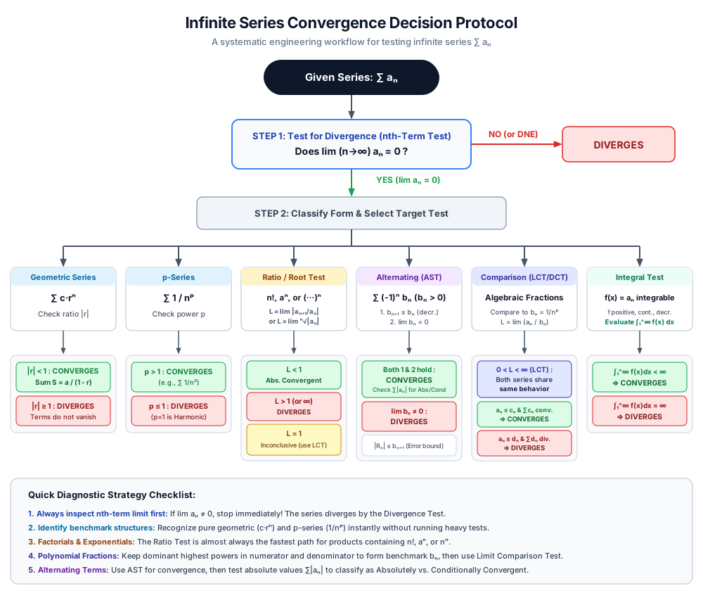
Series Convergence Tests Decision Flowchart

Power Series, Taylor & Maclaurin Expansions

  • Taylor Series about x=ax = a:
    f(x)=∑n=0∞f(n)(a)n!(x−a)n=f(a)+f′(a)(x−a)+f′′(a)2!(x−a)2+⋯f(x) = \sum_{n=0}^{\infty} \frac{f^{(n)}(a)}{n!}(x - a)^n = f(a) + f'(a)(x - a) + \frac{f''(a)}{2!}(x - a)^2 + \cdots
  • Maclaurin Series (a=0a = 0): f(x)=∑n=0∞f(n)(0)n!xnf(x) = \sum_{n=0}^{\infty} \frac{f^{(n)}(0)}{n!}x^n
  • Standard Maclaurin Series:
    11−x=∑n=0∞xn=1+x+x2+x3+⋯(∣x∣<1)\frac{1}{1 - x} = \sum_{n=0}^{\infty} x^n = 1 + x + x^2 + x^3 + \cdots \quad (|x| < 1)
    ex=∑n=0∞xnn!=1+x+x22!+x33!+⋯(−∞<x<∞)e^x = \sum_{n=0}^{\infty} \frac{x^n}{n!} = 1 + x + \frac{x^2}{2!} + \frac{x^3}{3!} + \cdots \quad (-\infty < x < \infty)
    sin⁡x=∑n=0∞(−1)nx2n+1(2n+1)!=x−x33!+x55!−⋯(−∞<x<∞)\sin x = \sum_{n=0}^{\infty} (-1)^n \frac{x^{2n+1}}{(2n+1)!} = x - \frac{x^3}{3!} + \frac{x^5}{5!} - \cdots \quad (-\infty < x < \infty)
    cos⁡x=∑n=0∞(−1)nx2n(2n)!=1−x22!+x44!−⋯(−∞<x<∞)\cos x = \sum_{n=0}^{\infty} (-1)^n \frac{x^{2n}}{(2n)!} = 1 - \frac{x^2}{2!} + \frac{x^4}{4!} - \cdots \quad (-\infty < x < \infty)
    ln⁡(1+x)=∑n=1∞(−1)n−1xnn=x−x22+x33−⋯(−1<x≤1)\ln(1 + x) = \sum_{n=1}^{\infty} (-1)^{n-1} \frac{x^n}{n} = x - \frac{x^2}{2} + \frac{x^3}{3} - \cdots \quad (-1 < x \le 1)
    arctan⁡x=∑n=0∞(−1)nx2n+12n+1=x−x33+x55−⋯(−1≤x≤1)\arctan x = \sum_{n=0}^{\infty} (-1)^n \frac{x^{2n+1}}{2n+1} = x - \frac{x^3}{3} + \frac{x^5}{5} - \cdots \quad (-1 \le x \le 1)
    (1+x)k=1+kx+k(k−1)2!x2+k(k−1)(k−2)3!x3+⋯(∣x∣<1)(1 + x)^k = 1 + kx + \frac{k(k-1)}{2!}x^2 + \frac{k(k-1)(k-2)}{3!}x^3 + \cdots \quad (|x| < 1)

4. Calculus III (Multivariable & Vector Calculus for Engineers)

4.1 3D Coordinate Geometry & Vectors

  • 3D Distance Formula: d=(x2−x1)2+(y2−y1)2+(z2−z1)2d = \sqrt{(x_2 - x_1)^2 + (y_2 - y_1)^2 + (z_2 - z_1)^2}
  • Sphere Equation: (x−x0)2+(y−y0)2+(z−z0)2=R2(x - x_0)^2 + (y - y_0)^2 + (z - z_0)^2 = R^2
  • Magnitude & Unit Vector:
    ∥v⃗∥=v12+v22+v32,u^=v⃗∥v⃗∥\|\vec{v}\| = \sqrt{v_1^2 + v_2^2 + v_3^2}, \quad \hat{u} = \frac{\vec{v}}{\|\vec{v}\|}
  • Dot Product:
    u⃗⋅v⃗=u1v1+u2v2+u3v3=∥u⃗∥∥v⃗∥cos⁡θ\vec{u} \cdot \vec{v} = u_1 v_1 + u_2 v_2 + u_3 v_3 = \|\vec{u}\|\|\vec{v}\|\cos\theta
    • Orthogonality Condition: u⃗⊥v⃗  ⟺  u⃗⋅v⃗=0\vec{u} \perp \vec{v} \iff \vec{u} \cdot \vec{v} = 0
    • Angle: cos⁡θ=u⃗⋅v⃗∥u⃗∥∥v⃗∥\cos\theta = \frac{\vec{u} \cdot \vec{v}}{\|\vec{u}\|\|\vec{v}\|}
  • Scalar & Vector Projections:
    scalu⃗v⃗=u⃗⋅v⃗∥u⃗∥\text{scal}_{\vec{u}}\vec{v} = \frac{\vec{u} \cdot \vec{v}}{\|\vec{u}\|}
    proju⃗v⃗=(u⃗⋅v⃗∥u⃗∥2)u⃗=(u⃗⋅v⃗u⃗⋅u⃗)u⃗\text{proj}_{\vec{u}}\vec{v} = \left(\frac{\vec{u} \cdot \vec{v}}{\|\vec{u}\|^2}\right)\vec{u} = \left(\frac{\vec{u} \cdot \vec{v}}{\vec{u} \cdot \vec{u}}\right)\vec{u}
    orthu⃗v⃗=v⃗−proju⃗v⃗\text{orth}_{\vec{u}}\vec{v} = \vec{v} - \text{proj}_{\vec{u}}\vec{v}
  • Cross Product:
    u⃗×v⃗=∣i^j^k^u1u2u3v1v2v3∣=⟨u2v3−u3v2,  u3v1−u1v3,  u1v2−u2v1⟩\vec{u} \times \vec{v} = \begin{vmatrix} \hat{i} & \hat{j} & \hat{k} \\ u_1 & u_2 & u_3 \\ v_1 & v_2 & v_3 \end{vmatrix} = \langle u_2 v_3 - u_3 v_2, \; u_3 v_1 - u_1 v_3, \; u_1 v_2 - u_2 v_1 \rangle
    • Magnitude: ∥u⃗×v⃗∥=∥u⃗∥∥v⃗∥sin⁡θ\|\vec{u} \times \vec{v}\| = \|\vec{u}\|\|\vec{v}\|\sin\theta
    • Parallel Condition: u⃗∥v⃗  ⟺  u⃗×v⃗=0⃗\vec{u} \parallel \vec{v} \iff \vec{u} \times \vec{v} = \vec{0}
    • Geometric Area of Parallelogram =∥u⃗×v⃗∥= \|\vec{u} \times \vec{v}\|; Area of Triangle =12∥u⃗×v⃗∥= \frac{1}{2}\|\vec{u} \times \vec{v}\|
    • Torque: τ⃗=r⃗×F⃗\vec{\tau} = \vec{r} \times \vec{F}
  • Triple Scalar Product & Volume:
    u⃗⋅(v⃗×w⃗)=∣u1u2u3v1v2v3w1w2w3∣\vec{u} \cdot (\vec{v} \times \vec{w}) = \begin{vmatrix} u_1 & u_2 & u_3 \\ v_1 & v_2 & v_3 \\ w_1 & w_2 & w_3 \end{vmatrix}
    • Parallelepiped Volume: V=∣u⃗⋅(v⃗×w⃗)∣V = |\vec{u} \cdot (\vec{v} \times \vec{w})|
    • Coplanarity Condition: u⃗,v⃗,w⃗\vec{u}, \vec{v}, \vec{w} are coplanar   ⟺  u⃗⋅(v⃗×w⃗)=0\iff \vec{u} \cdot (\vec{v} \times \vec{w}) = 0

4.2 Lines & Distances in 3D Space

  • Equations of a Line through P0(x0,y0,z0)P_0(x_0, y_0, z_0) with Direction v⃗=⟨a,b,c⟩\vec{v} = \langle a, b, c \rangle:
    • Vector Equation: r⃗(t)=r⃗0+tv⃗=⟨x0+at,y0+bt,z0+ct⟩\vec{r}(t) = \vec{r}_0 + t\vec{v} = \langle x_0 + at, y_0 + bt, z_0 + ct \rangle
    • Parametric Equations: x=x0+at,y=y0+bt,z=z0+ctx = x_0 + at, \quad y = y_0 + bt, \quad z = z_0 + ct
    • Symmetric Equations: x−x0a=y−y0b=z−z0c(abc≠0)\frac{x - x_0}{a} = \frac{y - y_0}{b} = \frac{z - z_0}{c} \quad (abc \ne 0)
  • Shortest Distance from Point MM to Line LL (Point P∈LP \in L, Direction v⃗\vec{v}):
    d=∥PM⃗×v⃗∥∥v⃗∥d = \frac{\|\vec{PM} \times \vec{v}\|}{\|\vec{v}\|}
  • Classification of Two 3D Lines L1(r⃗1(t)=r⃗01+tv⃗1)L_1(\vec{r}_1(t) = \vec{r}_{01} + t\vec{v}_1) and L2(r⃗2(s)=r⃗02+sv⃗2)L_2(\vec{r}_2(s) = \vec{r}_{02} + s\vec{v}_2):
    1. Parallel: v⃗1=kv⃗2\vec{v}_1 = k\vec{v}_2. (Coincident if points on L1L_1 satisfy L2L_2, otherwise Distinct Parallel).
    2. Intersecting: v⃗1≠kv⃗2\vec{v}_1 \ne k\vec{v}_2 and the linear system r⃗1(t)=r⃗2(s)\vec{r}_1(t) = \vec{r}_2(s) has a consistent unique solution (t∗,s∗)(t^*, s^*).
    3. Skew: v⃗1≠kv⃗2\vec{v}_1 \ne k\vec{v}_2 and the linear system r⃗1(t)=r⃗2(s)\vec{r}_1(t) = \vec{r}_2(s) is inconsistent (lines are non-parallel and non-intersecting).

4.3 Vector-Valued Functions, Curves, & Kinematics

  • Kinematic Hierarchy:
    • Position: r⃗(t)=⟨x(t),y(t),z(t)⟩\vec{r}(t) = \langle x(t), y(t), z(t) \rangle
    • Velocity: v⃗(t)=r⃗′(t)=⟨x′(t),y′(t),z′(t)⟩\vec{v}(t) = \vec{r}'(t) = \langle x'(t), y'(t), z'(t) \rangle
    • Acceleration: a⃗(t)=r⃗′′(t)=v⃗′(t)=⟨x′′(t),y′′(t),z′′(t)⟩\vec{a}(t) = \vec{r}''(t) = \vec{v}'(t) = \langle x''(t), y''(t), z''(t) \rangle
    • Scalar Speed: v(t)=∥v⃗(t)∥=(x′)2+(y′)2+(z′)2v(t) = \|\vec{v}(t)\| = \sqrt{(x')^2 + (y')^2 + (z')^2}
  • Arc Length & Intrinsic Parametrization:
    • Arc Length Integral: s=∫ab∥r⃗′(t)∥ dts = \int_{a}^{b} \|\vec{r}'(t)\|\,dt
    • Accumulated Arc Length Function: s(t)=∫at∥r⃗′(u)∥ du  ⟹  dsdt=∥r⃗′(t)∥s(t) = \int_{a}^{t} \|\vec{r}'(u)\|\,du \implies \frac{ds}{dt} = \|\vec{r}'(t)\|
    • Unit Speed Property under r⃗(s)\vec{r}(s): ∥r⃗′(s)∥=1\|\vec{r}'(s)\| = 1
  • TNB Frame & Curvature:
    • Unit Tangent Vector: T^(t)=r⃗′(t)∥r⃗′(t)∥\hat{T}(t) = \frac{\vec{r}'(t)}{\|\vec{r}'(t)\|}
    • Principal Unit Normal Vector: N^(t)=T^′(t)∥T^′(t)∥\hat{N}(t) = \frac{\hat{T}'(t)}{\|\hat{T}'(t)\|}
    • Binormal Vector: B^(t)=T^(t)×N^(t)\hat{B}(t) = \hat{T}(t) \times \hat{N}(t)
    • Curvature Formulas:
      κ=∥T^′(t)∥∥r⃗′(t)∥=∥r⃗′(t)×r⃗′′(t)∥∥r⃗′(t)∥3=∥v⃗×a⃗∥v3\kappa = \frac{\|\hat{T}'(t)\|}{\|\vec{r}'(t)\|} = \frac{\|\vec{r}'(t) \times \vec{r}''(t)\|}{\|\vec{r}'(t)\|^3} = \frac{\|\vec{v} \times \vec{a}\|}{v^3}
      For planar curve y=f(x)y = f(x): κ(x)=∣f′′(x)∣[1+(f′(x))2]3/2\kappa(x) = \frac{|f''(x)|}{[1 + (f'(x))^2]^{3/2}}
    • Radius of Curvature & Osculating Circle: ρ=1κ\rho = \frac{1}{\kappa}
  • Tangential & Normal Acceleration Decomposition:
    a⃗(t)=aTT^(t)+aNN^(t)\vec{a}(t) = a_T \hat{T}(t) + a_N \hat{N}(t)
    aT=ddt∥v⃗∥=v⃗⋅a⃗∥v⃗∥a_T = \frac{d}{dt}\|\vec{v}\| = \frac{\vec{v} \cdot \vec{a}}{\|\vec{v}\|}
    aN=κ∥v⃗∥2=∥v⃗×a⃗∥∥v⃗∥=∥a⃗∥2−aT2(aN≥0)a_N = \kappa \|\vec{v}\|^2 = \frac{\|\vec{v} \times \vec{a}\|}{\|\vec{v}\|} = \sqrt{\|\vec{a}\|^2 - a_T^2} \quad (a_N \ge 0)

4.4 Multivariable Differential Calculus

  • Partial Derivatives: fx=∂f∂x=lim⁡h→0f(x+h,y)−f(x,y)h,fy=∂f∂y=lim⁡h→0f(x,y+h)−f(x,y)hf_x = \frac{\partial f}{\partial x} = \lim_{h \to 0}\frac{f(x+h, y) - f(x,y)}{h}, \quad f_y = \frac{\partial f}{\partial y} = \lim_{h \to 0}\frac{f(x, y+h) - f(x,y)}{h}
  • Clairaut's Theorem: If fxyf_{xy} and fyxf_{yx} are continuous, then fxy=fyxf_{xy} = f_{yx}.
  • Tangent Plane to z=f(x,y)z = f(x,y) at (x0,y0,z0)(x_0, y_0, z_0):
    z−z0=fx(x0,y0)(x−x0)+fy(x0,y0)(y−y0)z - z_0 = f_x(x_0, y_0)(x - x_0) + f_y(x_0, y_0)(y - y_0)
  • Linear Approximation & Total Differential:
    L(x,y)=f(x0,y0)+fx(x0,y0)(x−x0)+fy(x0,y0)(y−y0)L(x,y) = f(x_0, y_0) + f_x(x_0, y_0)(x - x_0) + f_y(x_0, y_0)(y - y_0)
    dz=∂z∂xdx+∂z∂ydydz = \frac{\partial z}{\partial x}dx + \frac{\partial z}{\partial y}dy
  • Multivariable Chain Rule:
    • If z=f(x,y)z = f(x,y) where x=g(t),y=h(t)x = g(t), y = h(t): dzdt=∂z∂xdxdt+∂z∂ydydt\frac{dz}{dt} = \frac{\partial z}{\partial x}\frac{dx}{dt} + \frac{\partial z}{\partial y}\frac{dy}{dt}
    • If z=f(x,y)z = f(x,y) where x=g(u,v),y=h(u,v)x = g(u,v), y = h(u,v): ∂z∂u=∂z∂x∂x∂u+∂z∂y∂y∂u\frac{\partial z}{\partial u} = \frac{\partial z}{\partial x}\frac{\partial x}{\partial u} + \frac{\partial z}{\partial y}\frac{\partial y}{\partial u}
  • Gradient Vector & Directional Derivative:
    ∇f=⟨∂f∂x,∂f∂y,∂f∂z⟩\nabla f = \left\langle \frac{\partial f}{\partial x}, \frac{\partial f}{\partial y}, \frac{\partial f}{\partial z} \right\rangle
    Du^f=∇f⋅u^(∥u^∥=1)D_{\hat{u}}f = \nabla f \cdot \hat{u} \quad (\|\hat{u}\| = 1)
    • Maximum rate of increase is ∥∇f∥\|\nabla f\|, occurring in the direction of u^=∇f∥∇f∥\hat{u} = \frac{\nabla f}{\|\nabla f\|}.
    • Tangent plane to level surface F(x,y,z)=CF(x,y,z) = C at P0P_0: ∇F(P0)⋅⟨x−x0,y−y0,z−z0⟩=0\nabla F(P_0) \cdot \langle x - x_0, y - y_0, z - z_0 \rangle = 0.
  • Critical Points & Second Derivative Test:
    • Critical points occur where ∇f(x0,y0)=0⃗\nabla f(x_0, y_0) = \vec{0} or is undefined.
    • Discriminant: D=fxxfyy−(fxy)2D = f_{xx}f_{yy} - (f_{xy})^2
      • D>0 and fxx>0  ⟹  D > 0 \text{ and } f_{xx} > 0 \implies Local Minimum
      • D>0 and fxx<0  ⟹  D > 0 \text{ and } f_{xx} < 0 \implies Local Maximum
      • D<0  ⟹  D < 0 \implies Saddle Point
      • D=0  ⟹  D = 0 \implies Inconclusive
  • Lagrange Multipliers: To optimize f(x,y,z)f(x,y,z) subject to constraint g(x,y,z)=kg(x,y,z) = k:
    ∇f=λ∇gandg(x,y,z)=k\nabla f = \lambda \nabla g \quad \text{and} \quad g(x,y,z) = k

4.5 Multiple Integrals & Coordinate Transformations

  • Double Integrals:
    • Rectangular: ∬Rf(x,y) dA=∫ab∫cdf(x,y) dy dx\iint_R f(x,y)\,dA = \int_a^b \int_c^d f(x,y)\,dy\,dx
    • Polar Coordinates (x=rcos⁡θ,y=rsin⁡θ,x2+y2=r2x = r\cos\theta, y = r\sin\theta, x^2 + y^2 = r^2):
      ∬Rf(x,y) dA=∬Rf(rcos⁡θ,rsin⁡θ) r dr dθ\iint_R f(x,y)\,dA = \iint_R f(r\cos\theta, r\sin\theta)\,r\,dr\,d\theta
  • Triple Integrals:
    • Rectangular: dV=dx dy dzdV = dx\,dy\,dz
    • Cylindrical (x=rcos⁡θ,y=rsin⁡θ,z=zx = r\cos\theta, y = r\sin\theta, z = z):
      dV=r dr dθ dzdV = r\,dr\,d\theta\,dz
    • Spherical (x=ρsin⁡ϕcos⁡θ,y=ρsin⁡ϕsin⁡θ,z=ρcos⁡ϕ,x2+y2+z2=ρ2x = \rho\sin\phi\cos\theta, y = \rho\sin\phi\sin\theta, z = \rho\cos\phi, x^2 + y^2 + z^2 = \rho^2):
      dV=ρ2sin⁡ϕ dρ dϕ dθ(0≤ϕ≤π,  0≤θ≤2π)dV = \rho^2 \sin\phi\,d\rho\,d\phi\,d\theta \quad (0 \le \phi \le \pi, \; 0 \le \theta \le 2\pi)
  • Jacobian Transformation (2D & 3D):
    J(u,v)=∂(x,y)∂(u,v)=∣∂x∂u∂x∂v∂y∂u∂y∂v∣  ⟹  dA=∣J(u,v)∣ du dvJ(u,v) = \frac{\partial(x,y)}{\partial(u,v)} = \begin{vmatrix} \frac{\partial x}{\partial u} & \frac{\partial x}{\partial v} \\ \frac{\partial y}{\partial u} & \frac{\partial y}{\partial v} \end{vmatrix} \implies dA = |J(u,v)|\,du\,dv
  • Physical Applications of Multiple Integrals:
    • Mass: M=∬Dρ(x,y) dAorM=∭Eρ(x,y,z) dVM = \iint_D \rho(x,y)\,dA \quad \text{or} \quad M = \iiint_E \rho(x,y,z)\,dV
    • Center of Mass: xˉ=1M∬Dxρ dA,yˉ=1M∬Dyρ dA\bar{x} = \frac{1}{M}\iint_D x\rho\,dA, \quad \bar{y} = \frac{1}{M}\iint_D y\rho\,dA

4.6 Vector Calculus (Fields, Integrals, & Big Theorems)

  • Vector Field Operations:
    • Gradient: ∇f=⟨fx,fy,fz⟩\nabla f = \langle f_x, f_y, f_z \rangle
    • Divergence: div⁡F⃗=∇⋅F⃗=∂P∂x+∂Q∂y+∂R∂z\operatorname{div}\vec{F} = \nabla \cdot \vec{F} = \frac{\partial P}{\partial x} + \frac{\partial Q}{\partial y} + \frac{\partial R}{\partial z}
    • Curl: curl⁡F⃗=∇×F⃗=∣i^j^k^∂∂x∂∂y∂∂zPQR∣=⟨Ry−Qz,  Pz−Rx,  Qx−Py⟩\operatorname{curl}\vec{F} = \nabla \times \vec{F} = \begin{vmatrix} \hat{i} & \hat{j} & \hat{k} \\ \frac{\partial}{\partial x} & \frac{\partial}{\partial y} & \frac{\partial}{\partial z} \\ P & Q & R \end{vmatrix} = \left\langle R_y - Q_z, \; P_z - R_x, \; Q_x - P_y \right\rangle
    • Conservative Criterion: F⃗=∇f  ⟺  curl⁡F⃗=0⃗\vec{F} = \nabla f \iff \operatorname{curl}\vec{F} = \vec{0} (on simply connected domains).
  • Line Integrals:
    • Scalar: ∫Cf ds=∫abf(r⃗(t))∥r⃗′(t)∥ dt\int_C f\,ds = \int_a^b f(\vec{r}(t)) \|\vec{r}'(t)\|\,dt
    • Vector Work / Circulation: ∫CF⃗⋅dr⃗=∫abF⃗(r⃗(t))⋅r⃗′(t) dt=∫CP dx+Q dy+R dz\int_C \vec{F} \cdot d\vec{r} = \int_a^b \vec{F}(\vec{r}(t)) \cdot \vec{r}'(t)\,dt = \int_C P\,dx + Q\,dy + R\,dz
  • Fundamental Theorem for Line Integrals:
    ∫C∇f⋅dr⃗=f(r⃗(b))−f(r⃗(a))\int_C \nabla f \cdot d\vec{r} = f(\vec{r}(b)) - f(\vec{r}(a))
  • Green's Theorem (2D Plane):
    ∮CP dx+Q dy=∬D(∂Q∂x−∂P∂y) dA\oint_C P\,dx + Q\,dy = \iint_D \left( \frac{\partial Q}{\partial x} - \frac{\partial P}{\partial y} \right)\,dA
  • Surface Integrals:
    • Scalar: ∬Sf dS=∬Df(r⃗(u,v))∥r⃗u×r⃗v∥ dA\iint_S f\,dS = \iint_D f(\vec{r}(u,v)) \|\vec{r}_u \times \vec{r}_v\|\,dA
    • Vector Flux: ∬SF⃗⋅dS⃗=∬DF⃗(r⃗(u,v))⋅(r⃗u×r⃗v) dA\iint_S \vec{F} \cdot d\vec{S} = \iint_D \vec{F}(\vec{r}(u,v)) \cdot (\vec{r}_u \times \vec{r}_v)\,dA
  • Stokes' Theorem:
    ∮CF⃗⋅dr⃗=∬S(∇×F⃗)⋅dS⃗\oint_C \vec{F} \cdot d\vec{r} = \iint_S (\nabla \times \vec{F}) \cdot d\vec{S}
  • Divergence Theorem (Gauss's Theorem):
    ∬SF⃗⋅dS⃗=∭E(∇⋅F⃗) dV\iint_S \vec{F} \cdot d\vec{S} = \iiint_E (\nabla \cdot \vec{F})\,dV