Critical Points and Extrema
By the end of this session, you will be able to:
- Locate and classify critical numbers of polynomial, rational, and radical functions where f′(c)=0 or f′(c) is undefined (c∈dom(f)), distinguishing between extreme values (y) and locations (x), and applying Fermat's Theorem while recognizing that f′(c)=0 is a necessary but not sufficient condition for local extrema.
- Construct 1D derivative sign charts to analyze intervals of increase and decrease, and execute the First Derivative Test to classify local extrema and determine absolute extrema on open or unbounded intervals via the Single Critical Point Rule.
- Diagnose the hypotheses of the Extreme Value Theorem (EVT) (continuity on a closed interval [a,b]) and execute the 5-step Closed Interval Method Algorithm to locate absolute maxima and absolute minima across algebraic, logarithmic, and trigonometric functions.
📅 Micro-Lecture
1. Optimization Design & The Geometry of Critical Points
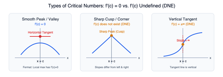
- Mathematical Foundation: An extreme value of a function represents an optimum: the greatest (maximum) or smallest (minimum) value achievable over a region. Calculus identifies candidate points by inspecting rates of change. A critical number of a function f is any value c in its domain (c∈dom(f)) where either the tangent is horizontal (f′(c)=0) or the curve experiences a sharp corner, cusp, or vertical tangent (f′(c) does not exist).
- Engineering Context: In civil, mechanical, and electrical engineering, locating critical points is the core engine of optimization. Structural engineers calculate zero-shear locations (dxdM=0) to locate maximum beam bending moments, aerospace engineers pinpoint peak dynamic pressure (q-Max) to size airframes, and electrical engineers locate peak transistor junction temperatures to avoid melting chip substrates.
2. Fermat's Theorem and the Converse Trap
- Mathematical Foundation: Fermat's Theorem states that if f has a local extremum at an interior point c and f′(c) exists, then f′(c)=0. However, students must avoid the classical Critical Number Converse Trap: f′(c)=0 does not guarantee an extremum. For example, f(x)=x3 has f′(0)=0, yet (0,0) is a flat inflection terrace—the function climbs continuously. To classify whether a critical number is a true local maximum, local minimum, or terrace, engineers construct a derivative sign chart and apply the First Derivative Test.
3. The Extreme Value Theorem & The Power of Preconditions
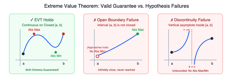
- Mathematical Foundation: Before investing computational effort into finding an optimum, engineers must confirm that an optimal solution actually exists. The Extreme Value Theorem (EVT) guarantees that if a function is continuous on a closed interval [a,b], it is mathematically guaranteed to attain both an absolute maximum and an absolute minimum. If either precondition fails (e.g., an open boundary marker or a vertical asymptote inside the interval), the guarantee vanishes, and the system may grow unbounded.
Skill Block 1
Real-Life Engineering Applications
Microchip Transistor Thermal Cycle Profiling (Electrical & Computer Engineering)
In high-power embedded electronics, autonomous robotics controllers, and server power supplies, gallium-nitride (GaN) high-electron-mobility transistors (HEMTs) switch high currents at megahertz frequencies. Rapid pulse-width modulation (PWM) switching induces dynamic thermal dissipation across the silicon-substrate junction.
An electronic systems engineer tests the thermal profile of a GaN power transistor during a scheduled 6-second operational duty cycle. Over the closed test interval t∈[0,6] seconds, the internal junction temperature T (in degrees Celsius, ∘C) is accurately modeled by the cubic polynomial:
To ensure hardware reliability and prevent catastrophic component failure, the hardware design team must audit the thermal operating limits against strict safety specifications:
- The maximum junction temperature rating of the silicon package is Tfail=125∘C. Exceeding this thermal ceiling triggers thermal runaway, melting internal bond wires.
- High-precision analog-to-digital signal calibration routines require minimal thermal noise interference, which occurs when the transistor is at its coolest operating point during the active cycle.
- Locate all critical numbers of the junction temperature function T(t) on the closed interval [0,6], and classify each critical number using the First Derivative Test.
- Determine the absolute maximum temperature and absolute minimum temperature reached during the duty cycle, identifying both the extreme values and their exact timing locations.
- Evaluate the component safety margin (Tfail−Tmax) and explain at what exact time instant firmware engineers should schedule precision sensor calibration to minimize thermal electronic noise.
💡 Show Worked Derivation
Problem Overview
We analyze the junction temperature T(t)=t3−9t2+15t+100 (∘C) of a power GaN transistor during a 6-second cycle (t∈[0,6]). We locate critical numbers, apply the First Derivative Test, determine absolute extrema using the Closed Interval Method, and audit hardware thermal safety and firmware calibration timing.
Step-by-Step Mathematical Solution
Step 1: Differentiate and Locate Critical Numbers
The governing formulation is the definition of Critical Numbers:
- Compute the first derivative using the Power Rule:
T′(t)=dtd[t3−9t2+15t+100]=3t2−18t+15
- Set T′(t)=0 to find stationary points:
3(t2−6t+5)=0Factoring the quadratic:3(t−1)(t−5)=0⟹t=1 sandt=5 s
- Check singular points: Since T′(t) is a polynomial, it is defined for all t.
- Both t=1 s and t=5 s lie strictly within the interior interval (0,6).
Step 2: Classify Critical Numbers via First Derivative Test
Construct a sign chart for T′(t)=3(t−1)(t−5) across the interval [0,6]:
- Interval (0,1): Test t=0.5⟹T′(0.5)=3(−0.5)(−4.5)=+6.75>0⟹(+). Temperature is increasing (↗).
- Interval (1,5): Test t=2⟹T′(2)=3(1)(−3)=−9<0⟹(−). Temperature is decreasing (↘).
- Interval (5,6): Test t=5.5⟹T′(5.5)=3(4.5)(0.5)=+6.75>0⟹(+). Temperature is increasing (↗).
Classification:
- At t=1 s: T′(t) changes sign from positive to negative (+→−). By the First Derivative Test, t=1 s is a local maximum.
- At t=5 s: T′(t) changes sign from negative to positive (−→+). By the First Derivative Test, t=5 s is a local minimum.
Step 3: Evaluate Candidate Values for Absolute Extrema
Using the Closed Interval Method Algorithm:
- Left Boundary (t=0 s):
T(0)=(0)3−9(0)2+15(0)+100=100∘C
- First Critical Point (t=1 s):
T(1)=(1)3−9(1)2+15(1)+100=1−9+15+100=107∘C
- Second Critical Point (t=5 s):
T(5)=(5)3−9(5)2+15(5)+100=125−225+75+100=75∘C
- Right Boundary (t=6 s):
T(6)=(6)3−9(6)2+15(6)+100=216−324+90+100=82∘C
Comparison:
- Absolute Maximum Temperature Value: 107∘C at location t=1 second.
- Absolute Minimum Temperature Value: 75∘C at location t=5 seconds.
Step 4: Engineering Analysis & Diagnostic Implications
- Safety Margin Audit:
The component thermal ceiling is Tfail=125∘C. The peak temperature is Tmax=107∘C.
Safety Margin=Tfail−Tmax=125∘C−107∘C=18∘CSince the margin is positive (18∘C>0), the transistor operates safely below its thermal breakdown threshold throughout the duty cycle.
- Firmware Calibration Scheduling: Johnson-Nyquist electronic thermal noise in semiconductor junctions is proportional to absolute temperature (vn2=4kBTRΔf). The global minimum temperature of 75∘C occurs at t=5 seconds. Firmware engineers should program the microcontroller to trigger high-precision ADC calibration sequences during the window surrounding t=5 seconds to ensure maximum signal-to-noise ratio (SNR).
Critical Numbers, Fermat's Theorem, and Local Extrema Classification
General Overview
Skill Block 1 establishes the mathematical grammar of optimization. Students learn to rigorously distinguish between an extreme value (y-coordinate) and its location (x-coordinate), enforce the Endpoint Rule (endpoints can never be relative extrema), locate critical numbers where f′(c)=0 or f′(c) is undefined, and avoid mistaking vertical asymptotes for critical numbers.
Conceptual Framework
- Extreme Values vs. Locations:
- The location is the input coordinate x=c.
- The extreme value is the function output height y=f(c).
- The extreme point is the ordered pair (c,f(c)) on the Cartesian grid.
- The Endpoint Rule:
- A relative (local) extremum requires an open neighborhood (c−δ,c+δ) centered at c that lies entirely within the domain of f.
- Because interval boundaries have domain points on only one side, domain endpoints can qualify as absolute extrema, but they are strictly disqualified from being relative extrema.
- The Domain Requirement for Critical Numbers:
- A number c is a critical number if and only if c∈dom(f) AND (f′(c)=0 or f′(c) DNE).
- Points of discontinuity (such as x=0 for f(x)=x1) are not critical numbers because they are excluded from the domain.
Key Equations & Structural Rules
- Critical Number Condition:
c∈dom(f)and[f′(c)=0orf′(c) DNE](see Critical Numbers and Critical Points)
- Fermat's Theorem on Local Extrema:
Local extremum at c⟹f′(c)=0(if f′(c) exists)(see Absolute and Relative Extrema)
Worked Example A: Classifying Extrema and Critical Numbers from Graphical Geometry
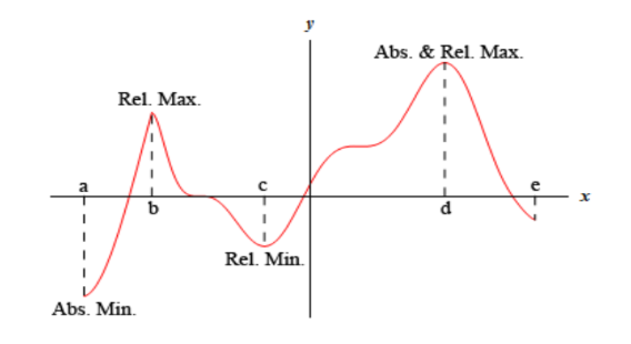
Given the graph of f(x) below defined over the closed interval [a,e], identify the locations and values of all absolute and relative extrema.
💡 Reveal Worked Solution
- Name the Governing Rules: The Definitions of Absolute and Relative Extrema and the Endpoint Rule: (These definitions are formalized in Absolute and Relative Extrema and Critical Numbers and Critical Points.)
- Identify Absolute Extrema (Global Highest and Lowest Heights):
- Absolute Maximum: Occurs at location x=d. The curve reaches its greatest vertical height across the entire domain [a,e] at the peak (d,f(d)).
- Absolute Minimum: Occurs at location x=a. The lowest point on the entire curve occurs at the left boundary endpoint (a,f(a)).
- Identify Relative (Local) Extrema (Interior Peaks and Valleys):
- Relative Maxima: Occur at locations x=b and x=d. In an open neighborhood around x=b, f(b)≥f(x), forming a local peak. Similarly, at x=d, f(d) is greater than all surrounding points.
- Relative Minimum: Occurs at location x=c. In an open interval around x=c, f(c)≤f(x), forming a local trough.
- Enforce the Endpoint Rule:
- The boundaries x=a and x=e are endpoints. Because they do not possess a two-sided open neighborhood within [a,e], they cannot be classified as relative extrema. The point x=a is strictly an absolute minimum, and x=e is neither.
Practice Problem 1: Concept & Reading Check
Open this Skill Block on the Memex to locate the information needed to answer the following:
- (a) In the Conceptual Framework, state the "Endpoint Rule." If a continuous function has its highest point at a boundary endpoint x=b, can x=b be classified as a relative maximum?
- (b) Deconstruct Worked Example A: Why is x=d classified as both a relative maximum and an absolute maximum, whereas x=b is classified only as a relative maximum?
- (c) Review the linked Engineering Application (Microchip Transistor Thermal Cycle Profiling (Electrical & Computer Engineering)). Why must electronic systems engineers calculate both the maximum value and the minimum value of junction temperature during a duty cycle?
Review the Endpoint Rule in the Conceptual Framework, compare heights at x=b and x=d in Worked Example A, and read the Problem Overview and Step 4 of Microchip Transistor Thermal Cycle Profiling (Electrical & Computer Engineering).
Answer: * (a) Relative extrema require a two-sided open neighborhood within the domain; endpoints have points on only one side and therefore can never be relative extrema.
- (b) x=d is an interior peak with a two-sided neighborhood (local max) and also achieves the highest function value on the entire interval (absolute max); x=b is a local peak but is exceeded by f(d).
- (c) The maximum temperature (107∘C) verifies safety against the thermal melting ceiling (125∘C); the minimum temperature (75∘C) identifies the exact low-noise timing window for sensor calibration.
Step-by-Step Execution
- (a) The Endpoint Rule states that relative (local) extrema can never occur at the endpoints of an interval because the definition of a relative extremum requires an open interval (c−δ,c+δ) centered at c lying entirely inside the domain. At an endpoint, function values exist on only one side. Therefore, while x=b can be the absolute maximum of the function on [a,b], it cannot be classified as a relative maximum.
- (b) In Worked Example A, location x=d lies in the interior of the interval [a,e] and is a turning point where f(d) is larger than all function values in an immediate two-sided open neighborhood, qualifying it as a relative maximum. Simultaneously, f(d) is the greatest function value across the entire interval, making it the absolute maximum. Location x=b is also an interior turning point higher than its immediate neighbors (so it is a relative maximum), but because f(b)<f(d), it does not attain the highest global value on the domain.
- (c) In GaN power transistor design, calculating the absolute maximum junction temperature (107∘C at t=1 s) confirms that the device maintains a safe 18∘C margin below its catastrophic melting ceiling of 125∘C. Calculating the absolute minimum temperature (75∘C at t=5 s) identifies the point of lowest thermal electronic noise (vn∝T), enabling firmware engineers to synchronize high-precision sensor calibration readings to this optimal temporal window.
Practice Problem 2
Consider the graph below defined over [−3,6]:
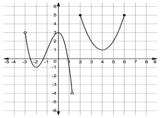
Identify all relative and absolute extrema (stating both values and locations), or explain why they do not exist:
- (a) Relative Maxima
- (b) Absolute Maximum
- (c) Relative Minima
- (d) Absolute Minimum
Review the definitions of Relative Extrema, Absolute Extrema, and the Endpoint Rule. Pay close attention to open circles versus solid dots on boundaries and branch terminations.
Answer: * (a) Relative Maxima: Value 3 at location x=0.
- (b) Absolute Maximum: Value 5 at locations x=2 and x=6.
- (c) Relative Minima: Value −1 at location x=−2, and Value 1 at location x=4.
- (d) Absolute Minimum: Does not exist (DNE).
Step-by-Step Execution
- Name the Governing Rules: Definition of Relative and Absolute Extrema: (These definitions are formalized in Absolute and Relative Extrema.)
- Evaluate Relative Maxima:
- At x=0, the curve reaches an interior peak with value f(0)=3. This is an interior turning point with a complete two-sided neighborhood, so the relative maximum value is 3 at x=0.
- The endpoints x=−3 and x=6 are disqualified by the Endpoint Rule. The point x=2 has domain values only for x≥2 because the left branch terminates at x≈1.25, so it has no two-sided neighborhood.
- Evaluate Absolute Maximum:
- The greatest function height reached on the graph is y=5.
- This value is attained at two locations: x=2 and x=6. Both coordinates have solid dots, confirming that the value 5 is achieved. Absolute maximum value is 5 at x=2 and x=6.
- Evaluate Relative Minima:
- At x=−2, the curve reaches an interior valley with value f(−2)=−1.
- At x=4, the curve reaches an interior valley with value f(4)=1.
- Both locations possess two-sided open neighborhoods where the point is lower than its immediate neighbors. Relative minima values are −1 at x=−2 and 1 at x=4.
- Evaluate Absolute Minimum:
- The graph approaches a low vertical height of −4 as x→1.25 on the left branch, but terminates in an open circle at (1.25,−4).
- Because this boundary point is excluded, the function values get arbitrarily close to −4 but never reach it. Since the function dips below all other valleys but never attains a minimum value, the absolute minimum does not exist (DNE).
Practice Problem 3
Find all critical numbers of the rational function on its domain:
State the Quotient Rule formula. Set f′(x)=0 to find stationary points and check where f′(x) is undefined. Verify each candidate against the domain of the original function.
Answer:
Step-by-Step Execution
- Name the Governing Formula: Quotient Rule and Definition of Critical Numbers:
dxd[vu]=v2u′v−uv′c∈dom(f)such thatf′(c)=0orf′(c) DNE(These definitions are formalized in Differentiation Rules - Basics, Powers, Products and Quotients and Critical Numbers and Critical Points.)
- Determine the Domain:
The rational function f(x) is defined for all real numbers except where the denominator is zero:
x−2=0⟹x=2dom(f)=(−∞,2)∪(2,∞)
- Compute the First Derivative:
Let u(x)=x2⟹u′(x)=2x, and v(x)=x−2⟹v′(x)=1:
f′(x)=(x−2)22x(x−2)−x2(1)=(x−2)22x2−4x−x2=(x−2)2x2−4x=(x−2)2x(x−4)
- Locate Stationary Points (f′(x)=0):
Set the numerator equal to zero:
x(x−4)=0⟹x=0orx=4Both x=0 and x=4 lie in the domain of f(x).
- Check Singular Points (f′(x) DNE):
The derivative is undefined when its denominator is zero:
(x−2)2=0⟹x=2However, x=2 is NOT in the domain of f(x) (f(2) is undefined; x=2 is a vertical asymptote). Therefore, x=2 cannot be a critical number.
- Conclusion: The critical numbers are strictly x=0 and x=4.
📅 Regroup 1
- Fermat's Theorem Converse Misconception: Emphasize that finding f′(c)=0 does not guarantee a local extremum. Show the cubic counterexample f(x)=x3 at x=0.
- The Domain Precondition: Reinforce that vertical asymptotes can never be critical numbers because critical numbers must belong to the domain of the function.
- Precision in Reporting: Review student answers to ensure they state x-values for locations and y-values for extreme values.
Skill Block 2
Real-Life Engineering Applications
Chemical Bioreactor Dissolved Oxygen Depletion (Chemical & Environmental Engineering)
In municipal wastewater treatment plants and pharmaceutical fermentation processes, aerobic microorganisms consume dissolved oxygen (DO) to break down organic contaminants. If dissolved oxygen drops too low, aerobic digestion halts; if aeration blowers run excessively, operational power consumption spikes.
An environmental engineer models the dissolved oxygen concentration C (in milligrams per liter, mg/L) inside a continuous stirred-tank bioreactor over time t (in hours, with t≥0) following a sudden organic shock loading:
- Using the Quotient Rule, determine the first derivative dtdC and find all critical numbers in the domain [0,∞).
- Construct a 1D derivative sign chart to determine the intervals on which dissolved oxygen is increasing and decreasing.
- Apply the First Derivative Test and the Single Critical Point Rule to determine the absolute maximum dissolved oxygen concentration and the exact time t at which this peak occurs.
- Determine the long-term asymptotic behavior limt→∞C(t) and explain why plant automation systems must restart supplemental aeration turbines once t exceeds the peak window.
💡 Show Worked Derivation
Problem Overview
We evaluate the dynamic dissolved oxygen profile C(t)=t2+48t (mg/L) for t≥0. We compute dtdC, construct a sign chart, apply the First Derivative Test and Single Critical Point Rule to find the global peak oxygen level, and assess aeration turbine controls.
Step-by-Step Mathematical Solution
Step 1: Differentiate via the Quotient Rule
The governing formulation is the Quotient Rule:
- Define numerator and denominator:
u(t)=8t⟹u′(t)=8v(t)=t2+4⟹v′(t)=2t
- Substitute into the Quotient Rule:
C′(t)=(t2+4)28(t2+4)−8t(2t)=(t2+4)28t2+32−16t2=(t2+4)232−8t2
- Factor the numerator:
C′(t)=(t2+4)28(4−t2)=(t2+4)28(2−t)(2+t)
Step 2: Locate and Filter Critical Numbers
The governing concept is Critical Numbers:
- Stationary Points (C′(t)=0):
Set the factored numerator to zero:
8(2−t)(2+t)=0⟹t=2ort=−2
- Domain Filter: The physical operational domain is t∈[0,∞). Therefore, t=−2 is discarded.
- Singular Points (C′(t) DNE): The denominator is (t2+4)2. Because t2+4≥4>0 for all real t, the denominator is never zero. There are no singular points.
- Valid Critical Number:
The function has exactly one critical number in its domain:
t=2 hours
Step 3: Construct Sign Chart & Apply First Derivative Test
Evaluate the sign of C′(t)=(t2+4)28(2−t)(2+t) on [0,∞) around t=2:
- Note that the denominator (t2+4)2>0 and the factor (2+t)>0 for all t>0. The sign is controlled strictly by (2−t).
- Interval (0,2): Test t=1⟹C′(1)=(1+4)28(1)(3)=2524>0⟹(+). Concentration is increasing (↗).
- Interval (2,∞): Test t=3⟹C′(3)=(9+4)28(−1)(5)=−16940<0⟹(−). Concentration is decreasing (↘).
Extremum Classification:
- Because C′(t) transitions from positive to negative (+→−) at t=2, C(2) is a local maximum.
- By the Single Critical Point Rule on [0,∞), because t=2 is the only interior critical number and C(0)=0, C(2) is guaranteed to be the absolute maximum over the entire domain:
C(2)=(2)2+48(2)=4+416=816=2.0 mg/L
- Absolute Maximum Value: 2.0 mg/L at location t=2 hours.
Step 4: Asymptotic Behavior & Operational Control
- Long-Term Limit:
Evaluate the limit as t→∞:
t→∞limC(t)=t→∞limt2+48t=t→∞lim1+4/t28/t=10=0 mg/L
- Process Engineering Control Decision: After the initial aeration surge reaches peak saturation (2.0 mg/L) at t=2 hours, active biological consumption drives the dissolved oxygen steadily downward toward zero. Environmental protection regulations require a minimum DO concentration of Cmin≥1.0 mg/L to prevent microbial die-off. Setting C(t)=1.0⟹t2+48t=1⟹t2−8t+4=0⟹t=4±23≈7.46 hours. Thus, the supervisory SCADA control system must automatically restart auxiliary air compressors before t≈7.46 hours.
The First Derivative Test and Monotonicity Sign Analysis
General Overview
Skill Block 2 equips students to construct 1D derivative sign charts to determine where functions are increasing or decreasing. Students apply the First Derivative Test to classify critical numbers as local maxima, local minima, or horizontal inflection terraces, and apply the Single Critical Point Rule to find global extrema on unbounded domains.
Conceptual Framework
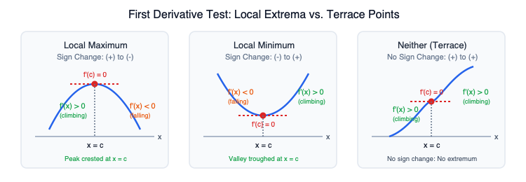
- The Monotonicity Test:
- f′(x)>0⟹f(x) is strictly increasing (↗).
- f′(x)<0⟹f(x) is strictly decreasing (↘).
- The First Derivative Test:
- Transition from (+) to (−) at c⟹f(c) is a local maximum (peak).
- Transition from (−) to (+) at c⟹f(c) is a local minimum (valley).
- Same sign on both sides of c⟹f(c) is neither (terrace point).
- The Single Critical Point Rule:
- If f(x) is continuous on an open or unbounded interval and contains exactly one critical number c:
- If f(c) is a local minimum, it is automatically the absolute minimum over the entire interval.
- If f(c) is a local maximum, it is automatically the absolute maximum over the entire interval.
- If f(x) is continuous on an open or unbounded interval and contains exactly one critical number c:
Key Equations & Structural Rules
- First Derivative Test Sign Transition Rules:
f′(x) changes (+)→(−)⟹Local Max at cf′(x) changes (−)→(+)⟹Local Min at c(see First Derivative Test)
- The Single Critical Point Rule on Interval I:
Exactly one critical number c∈I⟹Local Extremum is the Absolute Extremum(see First Derivative Test)
Worked Example A: First Derivative Test and the Single Critical Point Rule on an Open Domain
Find and classify all local and absolute extrema of the function:
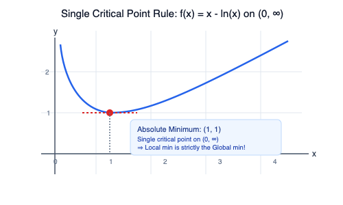
💡 Reveal Worked Solution
- Name the Governing Rule: The First Derivative Test and Single Critical Point Rule: (These rules are defined in First Derivative Test.)
- Compute the First Derivative:
Differentiating term by term:
f′(x)=dxd[x]−dxd[lnx]=1−x1=xx−1
- Locate Critical Numbers:
- Stationary point (f′(x)=0):
xx−1=0⟹x−1=0⟹x=1
- Singular point (f′(x) DNE): x=0, but 0∈/(0,∞).
- Thus, x=1 is the sole interior critical number.
- Stationary point (f′(x)=0):
- Construct the 1D Sign Chart:
Partition (0,∞) at x=1 into two test intervals:
- Interval (0,1): Choose test value x=0.5:
f′(0.5)=1−0.51=1−2=−1<0⟹(−)f(x) is decreasing on (0,1).
- Interval (1,∞): Choose test value x=2:
f′(2)=1−21=0.5>0⟹(+)f(x) is increasing on (1,∞).
- Interval (0,1): Choose test value x=0.5:
- Classify Extrema & Apply Single Critical Point Rule:
- Because f′(x) changes sign from negative to positive (−→+) at x=1, f(1) is a local minimum.
- By the Single Critical Point Rule, because x=1 is the only critical number in the entire open interval (0,∞), this local minimum is strictly the absolute minimum:
f(1)=1−ln(1)=1−0=1
- Absolute Minimum Value: 1 at location x=1.
- Absolute Maximum: Does not exist (as x→0+, −lnx→∞; as x→∞, x→∞).
Practice Problem 4: Concept & Reading Check
Open this Skill Block on the Memex to locate the information needed to answer the following:
- (a) In the Conceptual Framework, explain why test values must be substituted strictly into the derivative f′(x) rather than the original function f(x) during sign analysis.
- (b) Deconstruct Worked Example A: Why does the presence of only a single critical number on (0,∞) allow us to conclude that f(1)=1 is an absolute minimum without needing to test endpoints?
- (c) Review the linked Engineering Application (Chemical Bioreactor Dissolved Oxygen Depletion (Chemical & Environmental Engineering)). At what time does dissolved oxygen peak, and what mathematical theorem justifies that this peak is global?
Review the Sign Analysis Workflow in the Conceptual Framework, read Step 5 of Worked Example A, and inspect Step 3 of Chemical Bioreactor Dissolved Oxygen Depletion (Chemical & Environmental Engineering).
Answer: * (a) The sign of f′(x) reveals slope/direction (increasing vs. decreasing); substituting into f(x) only yields height, which reveals nothing about direction.
- (b) With no other critical points or asymptotes to turn the curve downward, a function that decreases to x=1 and increases thereafter can never achieve a value lower than f(1).
- (c) Peak occurs at t=2 hours (C(2)=2.0 mg/L); justified by the Single Critical Point Rule on [0,∞).
Step-by-Step Execution
- (a) Sign analysis determines the directional trajectory of a curve (whether it is climbing or falling). By the Monotonicity Theorem, the algebraic sign of the first derivative f′(x) dictates this slope (f′>0 means increasing; f′<0 means decreasing). Substituting a test value into the original function f(x) produces only the vertical height of the curve at that point, which provides zero information regarding whether the curve is sloping upward or downward.
- (b) In Worked Example A, the domain is the open interval (0,∞). Because f(x) is continuous and x=1 is the only critical number, the derivative f′(x) cannot change sign anywhere else. Since f′(x)<0 for all x∈(0,1) and f′(x)>0 for all x∈(1,∞), the curve descends monotonically to x=1 and ascends monotonically forever after. It is geometrically impossible for the function to turn back down to achieve a lower value, guaranteeing that the local minimum at x=1 is the global (absolute) minimum.
- (c) In the wastewater bioreactor model, dissolved oxygen reaches its maximum concentration of C(2)=2.0 mg/L at location t=2 hours. Because t=2 is the unique interior critical number on the operational domain [0,∞) and C′(t) transitions from positive to negative, the Single Critical Point Rule rigorously proves that 2.0 mg/L is the absolute maximum concentration attainable before supplemental blowers must restart.
Practice Problem 5
Find and classify all local extrema and determine any absolute extrema for the polynomial:
Differentiate using the Power Rule and factor out 30x4. Construct a sign chart testing intervals around x=0 and x=1. Evaluate end behavior as x→±∞.
Answer:
Step-by-Step Execution
- Name the Governing Formula: Power Rule and First Derivative Test:
dxd[xn]=nxn−1(These rules are defined in Differentiation Rules - Basics, Powers, Products and Quotients and First Derivative Test.)
- Compute the Derivative and Factor:
g′(x)=30x5−30x4=30x4(x−1)
- Locate Critical Numbers:
Setting g′(x)=0:
30x4(x−1)=0⟹x=0andx=1
- Construct 1D Sign Chart:
The critical numbers partition (−∞,∞) into (−∞,0), (0,1), and (1,∞). Note that 30x4>0 for all x=0:
- Interval (−∞,0): Test x=−1⟹g′(−1)=30(−1)4(−2)=−60<0⟹(−). Decreasing.
- Interval (0,1): Test x=0.5⟹g′(0.5)=30(0.5)4(−0.5)<0⟹(−). Decreasing.
- Interval (1,∞): Test x=2⟹g′(2)=30(2)4(1)=480>0⟹(+). Increasing.
- Classify Extrema:
- At x=0: g′(x) is negative on both sides. The curve flattens horizontally but continues falling. Thus, (0,3) is a terrace point (inflection point), neither a maximum nor a minimum.
- At x=1: g′(x) changes sign from negative to positive (−→+). Thus, g(1) is a local minimum:
g(1)=5(1)6−6(1)5+3=5−6+3=2
- Determine Absolute Extrema via End Behavior:
Because g(x) is an even-degree polynomial with a positive leading coefficient (5x6):
x→±∞limg(x)=∞Because the function diverges to +∞ on both boundaries, no absolute maximum exists. The local minimum of 2 at x=1 is the absolute minimum.
Practice Problem 6
Find and classify all critical points and absolute extrema of the function:
Differentiate using the Power Rule and Chain Rule. Look for points where the derivative is undefined. Evaluate end behavior as x→±∞.
Answer:
Step-by-Step Execution
- Name the Governing Formula: Chain Rule and Definition of Singular Critical Numbers:
dxd[u2/3]=32u−1/3⋅u′(These rules are defined in Chain Rule and Critical Numbers and Critical Points.)
- Compute the First Derivative:
h′(x)=−32(5−2x)−1/3⋅dxd[5−2x]=−3(5−2x)1/32⋅(−2)=3(5−2x)1/34
- Locate Critical Numbers:
- Stationary Points (h′(x)=0): The numerator is the constant 4=0. Therefore, h′(x)=0 everywhere.
- Singular Points (h′(x) DNE): The derivative is undefined when the denominator is zero:
3(5−2x)1/3=0⟹5−2x=0⟹x=25
- Since h(5/2)=7−(0)2/3=7, x=25 belongs to the domain and is a valid critical number (a sharp cusp).
- Construct 1D Sign Chart:
- Interval (−∞,5/2): Test x=0⟹h′(0)=3(5)1/34>0⟹(+). Increasing (↗).
- Interval (5/2,∞): Test x=3⟹h′(3)=3(5−6)1/34=3(−1)4=−34<0⟹(−). Decreasing (↘).
- Classify Extrema & End Behavior:
- Since h′(x) transitions from (+) to (−) at x=25, h(5/2)=7 is a local maximum.
- As x→±∞, (5−2x)2/3→+∞ because the power of 2/3 squares the quantity before taking the cube root. Thus:
x→±∞limh(x)=7−∞=−∞
- Since the curve descends infinitely on both ends, no absolute minimum exists.
- Absolute Maximum Value: 7 at location x=25.
📅 Regroup 2
- Testing Strictly in f′(x): Reiterate that when checking signs on a number line, test values must be substituted strictly into the derivative, not the original function.
- Handling Singular Critical Points: Emphasize that sharp cusps (f′(c) DNE) can be absolute extrema just like smooth stationary points (f′(c)=0).
- Single Critical Point Verification: Confirm students understand why the Single Critical Point Rule only works when there is exactly one critical point on the interval.
Skill Block 3
Real-Life Engineering Applications
Structural Beam Bending Moment Optimization (Civil & Construction Engineering)
In civil and construction engineering, horizontal reinforced concrete beams and steel girders spanning bridge roadways must withstand internal bending stresses induced by combined self-weight and dynamic traffic loads. Under standard beam bending theory, internal flexural fiber stress σ(x) is directly proportional to the internal bending moment M(x) across the beam cross-section:
A structural engineer evaluates a 6-meter long horizontal reinforced support beam across a closed building bay. The internal bending moment M (in kilonewton-meters, kN⋅m) at any horizontal position x (in meters from the left support wall) over the closed span x∈[0,6] is accurately modeled by:
- Verify that the hypotheses of the Extreme Value Theorem are satisfied for M(x) on [0,6].
- Compute M′(x) (the internal shear force distribution V(x)) and locate all interior critical numbers within (0,6).
- Execute the 5-step Closed Interval Method algorithm to determine the absolute maximum bending moment and absolute minimum bending moment, identifying both the extreme values and their exact longitudinal positions.
- Explain how the structural design engineer uses the calculated peak bending moment location to optimize steel rebar placement, detailing why placing heavy reinforcement uniformly across the entire 6-meter span would constitute costly construction waste.
💡 Show Worked Derivation
Problem Overview
We analyze the internal bending moment distribution M(x)=−2x3+15x2−24x+50 (kN⋅m) across a 6-meter span (x∈[0,6]). We verify the Extreme Value Theorem, locate critical points, execute the Closed Interval Method, and determine structural steel rebar placement to maximize safety while minimizing material costs.
Step-by-Step Mathematical Solution
Step 1: Verify Extreme Value Theorem Hypotheses
The governing theorem is the Extreme Value Theorem (EVT):
A continuous function on a closed interval [a,b] is guaranteed to achieve an absolute maximum and an absolute minimum. (This theorem is defined in Extreme Value Theorem.)
- Continuity: M(x) is a cubic polynomial. Polynomials are continuous for all real numbers R; hence M(x) is continuous on [0,6].
- Closed Domain: The domain [0,6] explicitly includes both structural support wall boundaries (x=0 and x=6).
- Conclusion: Both hypotheses are satisfied. Absolute extrema are guaranteed to exist.
Step 2: Differentiate and Locate Interior Critical Numbers
The governing concept is Critical Numbers:
- Differentiate using the Power Rule:
M′(x)=dxd[−2x3+15x2−24x+50]=−6x2+30x−24(In beam mechanics, the derivative of the bending moment is the internal shear force: V(x)=dxdM. Thus, critical points of the bending moment occur precisely where shear force is zero).
- Set M′(x)=0 to find stationary points:
−6(x2−5x+4)=0Factoring the quadratic:−6(x−1)(x−4)=0⟹x=1 mandx=4 m
- Check singular points: M′(x) is a polynomial, defined everywhere.
- Candidate Filtering: Both x=1 m and x=4 m lie strictly within the interior interval (0,6). Both are retained.
Step 3: Execute Candidate Height Evaluation (Closed Interval Method)
The governing algorithm is the Closed Interval Method: Evaluate the original bending moment function M(x) at all surviving interior critical numbers and boundary endpoints:
- Left Support Wall (x=0 m):
M(0)=−2(0)3+15(0)2−24(0)+50=50 kN⋅m
- First Critical Point (x=1 m):
M(1)=−2(1)3+15(1)2−24(1)+50=−2+15−24+50=39 kN⋅m
- Second Critical Point (x=4 m):
M(4)=−2(4)3+15(4)2−24(4)+50=−2(64)+15(16)−96+50M(4)=−128+240−96+50=66 kN⋅m
- Right Support Wall (x=6 m):
M(6)=−2(6)3+15(6)2−24(6)+50=−2(216)+15(36)−144+50M(6)=−432+540−144+50=14 kN⋅m
Step 4: Compare Heights and Identify Extrema
Comparing the four candidate values {50,39,66,14}:
- Absolute Maximum Bending Moment Value: 66 kN⋅m at location x=4 meters.
- Absolute Minimum Bending Moment Value: 14 kN⋅m at location x=6 meters.
Step 5: Civil Engineering Design Optimization
- Structural Safety and Rebar Clustering: The absolute peak bending moment of 66 kN⋅m represents the point of maximum tensile flexural stress in the concrete beam fibers. If structural failure occurs under dynamic loading, cracking will initiate at the bottom tensile face at x=4 meters. The civil engineer uses this calculus calculation to specify dense groupings of high-yield steel rebar stirrups and longitudinal tension bars concentrated in the zone around x=4 meters.
- Material Cost Savings vs. Uniform Sizing: At the right support wall (x=6 meters), the internal bending moment drops to its minimum of 14 kN⋅m—nearly 80% lower than the maximum. If an engineer lazily specified uniform maximum rebar reinforcement across the entire 6-meter span, the project would waste tons of expensive steel reinforcement in low-stress zones. By tapering rebar density according to the moment profile, construction costs are minimized while satisfying structural building codes.
The Extreme Value Theorem and The Closed Interval Method
General Overview
Skill Block 3 covers global optimization over bounded domains. Students verify the two preconditions of the Extreme Value Theorem (continuity and closed interval) and execute the 5-step Closed Interval Method Algorithm to locate absolute extrema across polynomial, logarithmic, and trigonometric functions.
Conceptual Framework
- The Extreme Value Theorem (EVT):
- If f(x) is continuous on a closed interval [a,b], it is guaranteed to attain both an absolute maximum and an absolute minimum value on [a,b].
- The 5-Step Closed Interval Method Algorithm:
- Check Preconditions: Verify continuity on [a,b].
- Differentiate: Compute f′(x).
- Find & Filter Interior Critical Numbers: Solve f′(c)=0 or undefined, retaining only c∈(a,b).
- Evaluate Original Heights: Compute f(a), f(b), and f(ci) for all surviving interior critical numbers.
- Compare: Greatest value is the absolute maximum; lowest value is the absolute minimum.
Key Equations & Structural Rules
- The Extreme Value Theorem:
f∈C[a,b]⟹∃c,d∈[a,b] such that f(c)≤f(x)≤f(d)∀x∈[a,b](see Extreme Value Theorem)
- Closed Interval Candidate Set:
Candidates={a,b}∪{c∈(a,b)∣f′(c)=0 or f′(c) DNE}(see Closed Interval Method)
Worked Example A: Closed Interval Method on a Cubic Polynomial
Find the absolute maximum and absolute minimum values of the function:
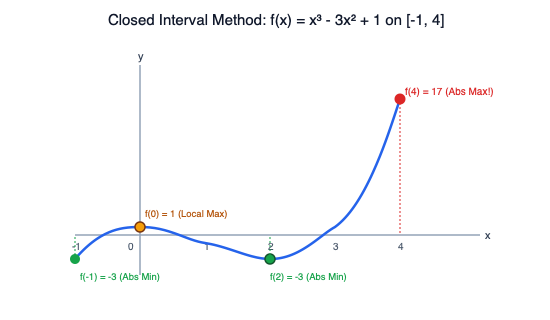
💡 Reveal Worked Solution
- Name the Governing Algorithm: The Closed Interval Method Algorithm: (This procedure is defined in Closed Interval Method and Extreme Value Theorem.)
- Step 1: Check Preconditions: f(x) is a cubic polynomial, which is continuous for all real numbers R. The domain [−1,4] is a closed, bounded interval. The Extreme Value Theorem is satisfied; absolute extrema are guaranteed.
- Step 2: Differentiate:
f′(x)=3x2−6x=3x(x−2)
- Step 3: Locate and Filter Interior Critical Numbers:
Set f′(x)=0:
3x(x−2)=0⟹x=0andx=2Filter Check: Both x=0 and x=2 lie strictly within the interior open interval (−1,4). Both are retained.
- Step 4: Evaluate the Original Function f(x) at All Candidates:
- Left Endpoint (x=−1):
f(−1)=(−1)3−3(−1)2+1=−1−3+1=−3
- First Critical Point (x=0):
f(0)=(0)3−3(0)2+1=1
- Second Critical Point (x=2):
f(2)=(2)3−3(2)2+1=8−12+1=−3
- Right Endpoint (x=4):
f(4)=(4)3−3(4)2+1=64−48+1=17
- Left Endpoint (x=−1):
- Step 5: Compare and Conclude:
Comparing candidate values {−3,1,−3,17}:
- Absolute Maximum Value: 17 at location x=4.
- Absolute Minimum Value: −3 at locations x=−1 and x=2.
Practice Problem 7: Concept & Reading Check
Open this Skill Block on the Memex to locate the information needed to answer the following:
- (a) In the Conceptual Framework, state the two required hypotheses of the Extreme Value Theorem. If a function is continuous on the interval (1,5], is it guaranteed to have an absolute minimum?
- (b) Deconstruct Worked Example A: Why did we evaluate f(−1) and f(4) even though f′(x)=0 at those points? What error occurs if an engineer evaluates f′(0) and f′(2) instead of f(0) and f(2) in Step 4?
- (c) Review the linked Engineering Application (Structural Beam Bending Moment Optimization (Civil & Construction Engineering)). At what location does the maximum bending moment occur, and how does this calculus result prevent construction waste?
Review the Two Pillars in the Conceptual Framework, inspect Step 4 and Pitfalls in Worked Example A, and read Step 3 and Step 5 of Structural Beam Bending Moment Optimization (Civil & Construction Engineering).
Answer: * (a) Hypotheses: (1) Continuity on interval, (2) Closed bounded interval [a,b]; for (1,5], the open left boundary means an absolute minimum is not guaranteed.
- (b) Absolute extrema can occur on boundary boundaries where slope is non-zero; evaluating f′ instead of f produces zero instead of the actual physical height.
- (c) Maximum moment of 66 kN⋅m occurs at x=4 m; engineers cluster steel rebar at x=4 m while tapering it at x=6 m (moment is only 14 kN⋅m), saving steel costs.
Step-by-Step Execution
- (a) The two hypotheses of the Extreme Value Theorem are: (1) The function must be continuous on the interval, and (2) The interval must be closed and bounded ([a,b]). If a function is defined on the half-open interval (1,5], it violates the closed interval hypothesis. As the function approaches x=1, it may drop toward a hole or asymptote without ever reaching a lowest included point. Therefore, an absolute minimum is not guaranteed to exist.
- (b) In Worked Example A, endpoints x=−1 and x=4 must be evaluated because the boundaries of a physical domain represent hard operational limits where the function may attain its global highest or lowest point without the derivative flattening to zero. If an engineer mistakenly substitutes critical numbers into the derivative f′(x) instead of the original function f(x), they obtain f′(0)=0 and f′(2)=0. This reports zero slope rather than the actual physical values (1 and −3), invalidating the entire comparison.
- (c) In structural beam design, the internal bending moment peaks at M(4)=66 kN⋅m at location x=4 meters. Because tensile flexural cracking initiates where bending moment peaks, civil engineers place dense steel rebar reinforcement specifically at the 4-meter mark. At the right support wall (x=6 meters), the moment drops to 14 kN⋅m. Tapering rebar reinforcement to match this moment distribution prevents the waste of tons of structural steel that would occur if maximum reinforcement were uniformly installed across the entire span.
Practice Problem 8
Determine whether the Extreme Value Theorem applies to the following functions on the given intervals. If it does not apply, identify which specific hypothesis failed:
- (a) f(x)=x−3x+2on [1,5]
- (b) g(x)=4x3−12xon (0,3]
Check both hypotheses of the Extreme Value Theorem: (1) Continuity across the entire interval, and (2) Fully closed interval boundaries.
Answer: * (a) EVT does not apply; violated hypothesis: Continuity (infinite discontinuity / vertical asymptote at x=3∈[1,5]).
- (b) EVT does not apply; violated hypothesis: Closed Interval (left boundary x=0 is open).
Step-by-Step Execution
- Name the Governing Theorem: Extreme Value Theorem Precondition Criteria: (This theorem is defined in Extreme Value Theorem.)
- Analysis for Part (a):
- Interval Check: [1,5] uses square brackets, so it is a closed interval.
- Continuity Check: f(x)=x−3x+2 has a denominator that equals zero when x−3=0⟹x=3. Because x=3 is in the interior of the interval [1,5], f(x) has an infinite discontinuity (vertical asymptote) inside the domain.
- Conclusion for (a): The EVT does not apply because f(x) fails the hypothesis of continuity on [1,5].
- Analysis for Part (b):
- Continuity Check: g(x)=4x3−12x is a polynomial, which is continuous everywhere on R.
- Interval Check: The domain is (0,3]. The left boundary at x=0 is indicated by a parenthesis, which excludes x=0.
- Conclusion for (b): The EVT does not apply because the interval is not closed.
Practice Problem 9
Find the absolute maximum and absolute minimum values and their locations for:
Differentiate using the Chain Rule dxd[lnu]=uu′. Set f′(x)=0 to find critical numbers. Evaluate candidate values at endpoints and critical numbers.
Answer:
Step-by-Step Execution
- Name the Governing Algorithm: Closed Interval Method with Chain Rule:
dxd[ln(u(x))]=u(x)u′(x)(This procedure is defined in Closed Interval Method and Chain Rule.)
- Step 1: Check Preconditions: The argument of the logarithm is x2+3x+4. Its discriminant is Δ=b2−4ac=9−16=−7<0. Because the discriminant is negative and the leading coefficient is positive, x2+3x+4>0 for all real x. Thus, f(x) is continuous everywhere on the closed interval [−2,2].
- Step 2: Differentiate:
f′(x)=x2+3x+42x+3
- Step 3: Locate and Filter Interior Critical Numbers:
Set f′(x)=0:
2x+3=0⟹x=−23=−1.5Since −1.5∈(−2,2), it is a valid interior critical number. (The denominator is never zero, so there are no singular points).
- Step 4: Evaluate f(x) at Candidates:
- Left Endpoint (x=−2):
f(−2)=ln((−2)2+3(−2)+4)=ln(4−6+4)=ln(2)≈0.693
- Interior Critical Point (x=−3/2):
f(−23)=ln((−23)2+3(−23)+4)=ln(49−29+4)=ln(47)≈0.560
- Right Endpoint (x=2):
f(2)=ln((2)2+3(2)+4)=ln(4+6+4)=ln(14)≈2.639
- Left Endpoint (x=−2):
- Step 5: Compare Results:
- Absolute Maximum Value: ln(14)≈2.639 at location x=2.
- Absolute Minimum Value: ln(47)≈0.560 at location x=−23.
Practice Problem 10
Find the absolute maximum and absolute minimum values and their locations for:
Simplify using the trigonometric identity cos(x+π/2)=−sin(x), or differentiate directly using the Chain Rule. Find critical numbers in (0,3π/2) and evaluate f(x) at all candidate points.
Answer:
Step-by-Step Execution
- Name the Governing Algorithm: Closed Interval Method for Trigonometric Functions: (This procedure is defined in Closed Interval Method.)
- Step 1: Simplify and Check Preconditions:
Using the co-function identity:
cos(x+2π)=−sin(x)The sine function is continuous everywhere on the closed interval [0,23π].
- Step 2 & 3: Differentiate and Find Critical Numbers:
f′(x)=−cos(x)Set f′(x)=0 on the interior interval (0,23π):−cos(x)=0⟹x=2πx=2π is the only interior critical number in (0,23π).
- Step 4: Evaluate f(x) at Candidates:
- Left Endpoint (x=0):
f(0)=−sin(0)=0
- Interior Critical Point (x=2π):
f(2π)=−sin(2π)=−1
- Right Endpoint (x=23π):
f(23π)=−sin(23π)=−(−1)=1
- Left Endpoint (x=0):
- Step 5: Compare Results:
- Absolute Maximum Value: 1 at location x=23π.
- Absolute Minimum Value: −1 at location x=2π.
Practice Problem 11
Find the absolute maximum and absolute minimum values and their locations for:
Differentiate using the Power Rule. Set g′(x)=0 to find stationary points and identify where g′(x) is undefined to find singular points. Evaluate g(x) at endpoints and all interior critical numbers.
Answer:
Step-by-Step Execution
- Name the Governing Algorithm: Closed Interval Method with Singular Points: (This procedure is defined in Closed Interval Method and Critical Numbers and Critical Points.)
- Step 1: Check Preconditions: g(x)=2x−3(3x)2 is continuous everywhere, including on [−1,8].
- Step 2: Differentiate:
g′(x)=2−3(32x−1/3)=2−x1/32=x1/32x1/3−2
- Step 3: Locate and Filter Interior Critical Numbers:
- Stationary Points (g′(x)=0): Numerator equals zero:
2x1/3−2=0⟹x1/3=1⟹x=1
- Singular Points (g′(x) DNE): Denominator equals zero:
x1/3=0⟹x=0
- Filter: Both x=0 and x=1 lie strictly inside the interior interval (−1,8).
- Stationary Points (g′(x)=0): Numerator equals zero:
- Step 4: Evaluate g(x) at All Candidates:
- Left Endpoint (x=−1):
g(−1)=2(−1)−3(−1)2/3=−2−3(1)=−5
- Singular Critical Point (x=0):
g(0)=2(0)−3(0)2/3=0
- Stationary Critical Point (x=1):
g(1)=2(1)−3(1)2/3=2−3=−1
- Right Endpoint (x=8):
g(8)=2(8)−3(8)2/3=16−3(4)=16−12=4
- Left Endpoint (x=−1):
- Step 5: Compare Results:
Comparing candidate heights {−5,0,−1,4}:
- Absolute Maximum Value: 4 at location x=8.
- Absolute Minimum Value: −5 at location x=−1.
📅 Regroup 3
- Evaluating in f(x) vs f′(x): Ensure every student understands why candidate heights are computed strictly in the original function f(x).
- Singular Points on Closed Intervals: Remind students to always check where the derivative denominator equals zero (singular points like x=0 in Problem 11).
- The Role of Endpoints: Emphasize that endpoints are equal-status candidates in global optimization and must never be skipped.
📅 Synthesis Wrap-up
- Connecting the Toolkit: Today we transitioned from understanding local behavior (where slopes flatten or peak via Fermat's Theorem and the First Derivative Test) to global optimization on closed intervals via the Extreme Value Theorem.
- Looking Ahead to Sessions 14 & 15: In upcoming sessions, we take this exact mathematical machinery and apply it to real-world geometric and kinematic design: finding the dimensions that maximize container volume or minimize pipeline construction cost (constrained optimization).
- Homework Preparation: Complete the Knewton Alta assignment Critical Points and Extrema. Ensure you check your domain restrictions and test signs carefully!