Session 06 - Rates of Change and the Definition of the Derivative

📅 Micro-Lecture

1. Rates of Change & The Secant-to-Tangent Transition

Mathematical Foundation: The average rate of change between two points on a curve corresponds to the slope of a secant line: $\frac{f(a+h)-f(a)}{h}$ (see Difference Quotient). As the interval width shrinks to zero ( $h \to 0$ ), the secant line rotates into the tangent line at $x = a$ . The limiting value of this difference quotient defines the instantaneous rate of change or derivative $f'(a)$ (see Derivatives).
Engineering Context: Kinematic tracking in automotive and aerospace vehicles computes instantaneous acceleration from high-frequency GPS position pings, while biomedical telemetry monitors instantaneous pulse rate spikes during cardiovascular stress testing.

2. Formal Differentiability & Structural Failure Modes

Mathematical Foundation: Differentiability at a point requires a finite, unique two-sided derivative limit. While differentiability guarantees continuity ( $\text{differentiable} \implies \text{continuous}$ ), continuity does not guarantee differentiability (see Differentiability). Differentiability fails visually at sharp corners, cusps, vertical tangents, and points of discontinuity (see Discontinuities).
Engineering Context: High-speed railway track junctions and highway ramps require continuous tangent slopes ( $C^1$ smoothness) to prevent violent lateral centrifugal acceleration spikes. In structural mechanics, internal sharp corners create non-differentiable stress concentration points where micro-cracks form, requiring smooth rounded fillets.

3. The Derivative Function & Tangent Line Linearization

Mathematical Foundation: Evaluating the difference quotient limit with respect to the variable $x$ yields the derivative function $f'(x)$ , which outputs the instantaneous slope at any point along the curve. This slope enables the construction of the tangent line $y - f(a) = f'(a)(x-a)$ (see Tangent Lines).
Engineering Context: Onboard autopilot flight controllers linearize complex non-linear aerodynamic flight dynamics around current operational waypoints, executing microsecond trajectory adjustments without overloading embedded processors.

Segment 1 of 8

Skill Block 1

Real-Life Engineering Applications

🏗️

Civil Engineering

Speed Railway Transition (Civil Engineering)

A transportation civil engineer is designing a track layout for a new high-speed passenger railway. The horizontal position profile of the track alignment transitions from a straight access track into a curved bypass, modeled by the piecewise function:

T(x) = \begin{cases} 2x & \text{for } x \le 3 \\ x^2 - 4x + 9 & \text{for } x > 3 \end{cases}

where

x

and

T(x)

are measured in hundreds of meters.

Analytically determine if the track layout is continuous at the junction point $x = 3$ .
Determine if the track layout is differentiable at $x = 3$ by comparing the left-hand and right-hand derivative limits.
Based on differentiability and lateral dynamics, explain why this transition geometry is either safe or hazardous for a passenger train traveling at high speeds.

💡 Show Worked Derivation

Problem Overview

We analyze the continuity and differentiability of the railway track alignment profile at the junction coordinate $x = 3$ :

T(x) = \begin{cases} 2x & x \le 3 \\ x^2 - 4x + 9 & x > 3 \end{cases}

Step-by-Step Mathematical Solution

Step 1: Check for Continuity at $x = 3$

Evaluate the left-hand limit, right-hand limit, and function value at $x = 3$ :

Left-hand limit: $\lim_{x \to 3^-} T(x) = \lim_{x \to 3^-} (2x) = 2(3) = 6$
Right-hand limit: $\lim_{x \to 3^+} T(x) = \lim_{x \to 3^+} (x^2 - 4x + 9) = (3)^2 - 4(3) + 9 = 9 - 12 + 9 = 6$
Function value: $T(3) = 2(3) = 6$

Since $\lim_{x \to 3^-} T(x) = \lim_{x \to 3^+} T(x) = T(3) = 6$ , the two track segments meet continuously at $(3, 6)$ without any physical gap.

Step 2: Check for Differentiability at $x = 3$

Compute the one-sided derivative limits approaching $x = 3$ :

Left-hand derivative (straight track): $\lim_{h \to 0^-} \frac{T(3+h) - T(3)}{h} = \lim_{h \to 0^-} \frac{2(3+h) - 6}{h} = \lim_{h \to 0^-} \frac{2h}{h} = 2$
Right-hand derivative (curved bypass): $\lim_{h \to 0^+} \frac{T(3+h) - T(3)}{h} = \lim_{h \to 0^+} \frac{[(3+h)^2 - 4(3+h) + 9] - 6}{h}$ $= \lim_{h \to 0^+} \frac{9 + 6h + h^2 - 12 - 4h + 9 - 6}{h} = \lim_{h \to 0^+} \frac{2h + h^2}{h} = \lim_{h \to 0^+} (2 + h) = 2$

Since the incoming tangent slope ( $2$ ) matches the outgoing tangent slope ( $2$ ), the function is differentiable at $x = 3$ with $T'(3) = 2$ .

Engineering Conclusion

Because the track profile is differentiable at $x = 3$ , the alignment forms a smooth curve without a sharp geometric corner ( $C^1$ continuity). This layout is safe for high-speed operation. If the one-sided slopes did not match (creating a non-differentiable corner), high-speed trains crossing the junction would experience an instantaneous impulse step in lateral acceleration and jerk, creating severe derailment risks and structural wheel-flange damage.

⚙️

Mechanical Engineering

Stress Concentration at Structural Notch (Mechanical Engineering)

A mechanical engineer conducts a finite element stress simulation on a critical titanium aerospace load-bearing bracket. The boundary geometry along the inner tension surface of the bracket is described by the absolute-value profile:

y(x) = |x - 5| + 2 \quad \text{for } x \in [0, 10]

where

x

represents the longitudinal position in centimeters and

y(x)

represents the surface contour.

Analytically prove that $y(x)$ is continuous but non-differentiable at the vertex $x = 5$ .
Explain the physical consequence of this geometric non-differentiability regarding stress concentration factors ( $K_t$ ) when the bracket is subjected to cyclic operational loads.
Propose the mathematical modification engineers implement (such as a circular or polynomial transition fillet) to restore differentiability and safeguard against fatigue crack initiation.

💡 Show Worked Derivation

Problem Overview

We analyze the geometric continuity, differentiability, and stress concentration characteristics of the V-notch profile:

y(x) = |x - 5| + 2

at the notch vertex

x = 5

.

Step-by-Step Mathematical Solution

Step 1: Prove Continuity at $x = 5$

Rewrite $y(x)$ as a piecewise function:

y(x) = \begin{cases} -(x - 5) + 2 = -x + 7 & x < 5 \\ (x - 5) + 2 = x - 3 & x \ge 5 \end{cases}

Left-hand limit: $\lim_{x \to 5^-} (-x + 7) = -5 + 7 = 2$
Right-hand limit: $\lim_{x \to 5^+} (x - 3) = 5 - 3 = 2$
Function value: $y(5) = |5 - 5| + 2 = 2$

Since $\lim_{x \to 5^-} y(x) = \lim_{x \to 5^+} y(x) = y(5) = 2$ , the bracket contour is continuous at $x = 5$ .

Step 2: Test for Differentiability at $x = 5$

Compute the one-sided derivative limits using the difference quotient:

Left-hand derivative: $\lim_{h \to 0^-} \frac{y(5+h) - y(5)}{h} = \lim_{h \to 0^-} \frac{|(5+h) - 5| + 2 - 2}{h} = \lim_{h \to 0^-} \frac{|h|}{h} = \lim_{h \to 0^-} \frac{-h}{h} = -1$
Right-hand derivative: $\lim_{h \to 0^+} \frac{y(5+h) - y(5)}{h} = \lim_{h \to 0^+} \frac{|h|}{h} = \lim_{h \to 0^+} \frac{h}{h} = +1$

Because $\lim_{h \to 0^-} \frac{\Delta y}{h} = -1 \neq +1 = \lim_{h \to 0^+} \frac{\Delta y}{h}$ , the two-sided limit does not exist. The function has a sharp corner and is non-differentiable at $x = 5$ .

Engineering Conclusion

In structural mechanics and elasticity theory, an abrupt geometric corner with zero radius of curvature ( $r \to 0$ ) causes the theoretical stress concentration factor $K_t = 1 + 2\sqrt{a/r}$ to approach infinity. Under dynamic cyclic service loads, physical stress lines crowd at this non-differentiable vertex, inducing localized plastic deformation and micro-crack nucleation.

To eliminate this catastrophic failure mode, mechanical engineers replace sharp corners with tangent transition arcs or smooth polynomial curves (fillets), ensuring that the geometric derivative $y'(x)$ remains continuous ( $C^1$ ) across the entire surface profile and distributing internal stresses uniformly.

📚 1. Core Theory 💡 2. Worked Example ✍️ 3. Active Practice

Average vs. Instantaneous Rates of Change and Differentiability

General Overview
Skill Block 1 establishes the geometric transition from secant line slopes (average rates) to tangent line slopes (instantaneous rates), and develops visual and analytic criteria for classifying where derivatives exist or fail.

Conceptual Framework

Secant Line vs. Tangent Line: A secant line connects two points $(a, f(a))$ and $(a+h, f(a+h))$ with slope $\frac{\Delta y}{\Delta x}$ . Taking $\lim_{h \to 0}$ collapses the two points into a single point of tangency, yielding the tangent slope $f'(a)$ (see Derivatives).
Differentiability Implies Continuity: If $f'(a)$ exists, then $\lim_{x \to a} f(x) = f(a)$ . If a function is discontinuous at $x = a$ , it cannot be differentiable at $a$ (see Continuity).
The Four Visual Signatures of Non-Differentiability:
1. Corner / Sharp Turn: Left-hand slope $\neq$ Right-hand slope ( $\lim_{h \to 0^-} \neq \lim_{h \to 0^+}$ ).
2. Cusp: Slopes approach opposite infinities ( $+\infty$ on one side, $-\infty$ on the other).
3. Vertical Tangent: The slope limit is infinite ( $\pm\infty$ ).
4. Discontinuity: A hole, step jump, or vertical asymptote breaks the curve.

Key Equations & Structural Rules

Average Rate of Change (ARoC): $\text{ARoC} = \frac{f(b) - f(a)}{b - a} = \frac{f(a+h) - f(a)}{h}$
Instantaneous Rate of Change (IRoC): $\text{IRoC} = f'(a) = \lim_{h \to 0} \frac{f(a+h) - f(a)}{h}$
Differentiability Condition: $f'(a)$ exists if and only if $\lim_{h \to 0^-} \frac{f(a+h)-f(a)}{h} = \lim_{h \to 0^+} \frac{f(a+h)-f(a)}{h} = L \in \mathbb{R}$ (see Differentiability).

Worked Example A: Graphical Derivative and Differentiability Analysis

Consider a piecewise function $g(x)$ defined on $[-6, 8]$ with a vertical asymptote at $x = -2$ , a sharp corner at $(1, 3)$ , a straight line segment connecting $(2, 0)$ to $(5, 6)$ , and a jump discontinuity at $x = 5$ from $(5, 6)$ to $(5, 2)$ .

(a) Evaluate $g'(4)$ .
(b) Identify all $x$ -values on $(-6, 8)$ where $g(x)$ is continuous but NOT differentiable.

💡 Reveal Worked Solution

Evaluate the derivative on the straight segment for $g'(4)$ : Notice that $x = 4$ lies on the straight line segment between $(2, 0)$ and $(5, 6)$ . On any linear segment, the instantaneous rate of change equals the constant slope of that segment: $g'(4) = \frac{y_2 - y_1}{x_2 - x_1} = \frac{6 - 0}{5 - 2} = \frac{6}{3} = 2$
Identify points where $g(x)$ is continuous but not differentiable: Scan for points where the curve is fully connected (continuous) yet has no unique non-vertical tangent line:
- At $x = -2$ , $g(x)$ has a vertical asymptote (discontinuous $\implies$ non-differentiable).
- At $x = 5$ , $g(x)$ has a jump discontinuity (discontinuous $\implies$ non-differentiable).
- At $x = 1$ , the graph forms a sharp V-shaped corner at $(1, 3)$ . The function is continuous because the left and right paths meet at $(1, 3)$ , but the left-hand incoming slope does not equal the right-hand outgoing slope.
Conclusion: $g(x)$ is continuous but non-differentiable at $x = 1$ .

Practice Problem 1: Concept & Reading Check

Open this Skill Block on the Memex to locate the information needed to answer the following:

(a) Under the Conceptual Framework section, explain why continuity is a necessary but not sufficient condition for differentiability.
(b) In Worked Example A, explain why the derivative $g'(4)$ can be calculated directly using the standard slope formula $\frac{y_2 - y_1}{x_2 - x_1}$ .
(c) Review the linked Engineering Applications ("High-Speed Railway Transition"). Why must the position profile of a high-speed railway track be differentiable ( $T'(3)$ exists) rather than merely continuous at track junctions?

Practice Space Solve this problem on paper or tablet.

Review the Conceptual Framework regarding the four failure modes of differentiability, check step 1 of Worked Example A, and refer to the engineering conclusion in High-Speed Railway Transition (Civil Engineering).

Answer: * (a) Differentiability requires the curve to be unbroken (continuous) AND smooth (having a single, finite non-vertical tangent slope). A function can be continuous but have sharp corners or vertical tangents where slopes fail to exist.

(b) Because $x = 4$ falls along a straight line segment, and the derivative (instantaneous slope) of any straight line is constant and equals the slope of the secant line across that interval.
(c) Differentiability guarantees that the incoming and outgoing track slopes match smoothly. A non-differentiable corner causes an instantaneous spike in lateral centrifugal force that can derail high-speed trains.

Step-by-Step Execution

(a) As detailed in the Conceptual Framework, the theorem $\text{differentiable} \implies \text{continuous}$ confirms that differentiability requires continuity. However, the converse is false because a curve may be connected without breaks (continuous) yet feature sharp corners, cusps, or vertical tangents where the two-sided limit of the difference quotient does not exist or is infinite.
(b) For any linear segment $y = mx + b$ , the difference quotient $\frac{g(4+h)-g(4)}{h} = \frac{[m(4+h)+b] - [m(4)+b]}{h} = \frac{mh}{h} = m$ is constant for all $h$ . Thus, evaluating the derivative at $x = 4$ simply equals the geometric slope $\frac{6-0}{5-2} = 2$ .
(c) In High-Speed Railway Transition (Civil Engineering), differentiability at $x = 3$ ensures that the straight track seamlessly aligns with the curved bypass with an identical tangent vector ( $T'(3) = 2$ ). If the derivatives mismatched, the resulting sharp corner would subject traveling train cars to infinite lateral jerk and severe centrifugal derailment hazards.

Practice Problem 2

Consider the graph of $f(x)$ given below:

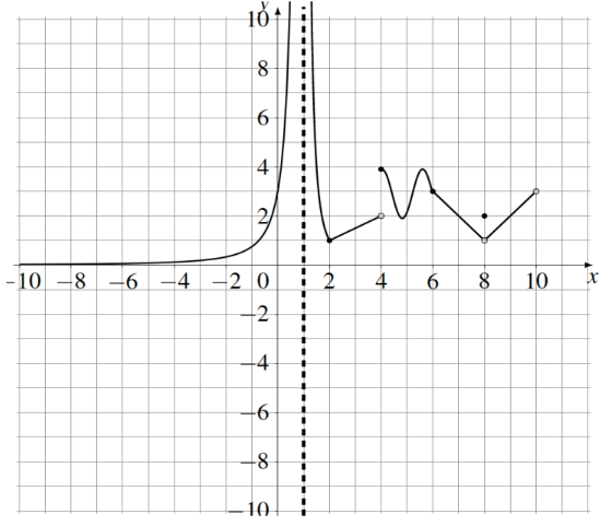
06 - Rates of Change and Definition of Derivative Learning Activity Image 1.png

(a) Find the following values:
- i. $\lim_{x\to 4} f(x)$
- ii. $\lim_{x\to 1^+} f(x)$
- iii. $\lim_{x\to 8} f(x)$
- iv. $\lim_{x\to 10^-} f(x)$
- v. $\lim_{x\to -\infty} f(x)$
- vi. $f'(3)$
(b) State any horizontal and vertical asymptotes for $f(x)$ .
(c) Identify any points of discontinuity for $f(x)$ AND indicate the type of discontinuity for each.
(d) At which points, if any, is $f(x)$ continuous but not differentiable? State the $x$ -value(s) and justify.

Practice Space Solve this problem on paper or tablet.

For limit values, inspect left and right approaches. For $f'(3)$ , locate $x = 3$ on the graph and find the slope of that straight line segment. For continuity without differentiability, look exclusively for unbroken sharp corners.

Answer: * (a) i. $\text{DNE}$ ; ii. $\infty$ ; iii. $1$ ; iv. $3$ ; v. $0$ ; vi. $\frac{1}{2}$

(b) Horizontal Asymptote: $y = 0$ (as $x \to -\infty$ ); Vertical Asymptote: $x = 1$ .
(c) $x = 1$ (Infinite), $x = 4$ (Jump), $x = 8$ (Removable).
(d) $x = 2$ and $x = 6$ (sharp corners where left and right slopes mismatch).

Step-by-Step Execution

(a) Graphical evaluations:
- i. $\lim_{x\to 4} f(x) = \text{DNE}$ because $\lim_{x\to 4^-} f(x) = 2 \neq 4 = \lim_{x\to 4^+} f(x)$ .
- ii. $\lim_{x\to 1^+} f(x) = \infty$ (curve rises indefinitely to the right of $x = 1$ ).
- iii. $\lim_{x\to 8} f(x) = 1$ (both paths approach the open hole at $y = 1$ ).
- iv. $\lim_{x\to 10^-} f(x) = 3$ (approaching the right endpoint).
- v. $\lim_{x\to -\infty} f(x) = 0$ (horizontal asymptote along the $x$ -axis).
- vi. $f'(3) = \frac{1}{2}$ because on $[2, 4]$ , the graph is a line segment through $(2, 1)$ and $(4, 2)$ : $\text{Slope} = \frac{2 - 1}{4 - 2} = \frac{1}{2}$ .
(b) Asymptotes: Horizontal asymptote at $y = 0$ as $x \to -\infty$ ; Vertical asymptote at $x = 1$ .
(c) Discontinuities:
- $x = 1$ : Infinite discontinuity (vertical asymptote).
- $x = 4$ : Jump discontinuity (one-sided limits are finite but unequal).
- $x = 8$ : Removable discontinuity (hole at $y = 1$ , with $f(8) = 2$ ).
(d) Continuous but Non-Differentiable:
- $x = 2$ and $x = 6$ : At both coordinates, the graph is continuous (unbroken), but forms a sharp corner where incoming and outgoing slopes change abruptly. (Note: $x = 1, 4, 8$ are also non-differentiable, but they fail continuity).

Segment 2 of 8

📅 Regroup 1

Clarify the geometric difference between secant lines and tangent lines.
Reiterate why continuity is necessary for differentiability, but not sufficient (highlighting sharp corners and cusps).

Segment 3 of 8

Skill Block 2

Real-Life Engineering Applications

⚡

Electrical Engineering

Inductor Transient Voltage (Electrical Engineering)

An electrical engineer tests a power regulation circuit containing a specialized high-frequency inductor with an inductance of $L = 0.5\text{ Henries}$ ( $0.5\text{ H}$ ). During a rapid switching transient, the time-varying current $i(t)$ (in Amperes) flowing through the inductor for $t > 0$ seconds follows the rational decay function:

i(t) = \frac{6}{t}

The fundamental physical constitutive relation governing the induced voltage $V_L(t)$ across an inductor is given by Faraday's law:

V_L(t) = L \cdot \frac{di}{dt}

Using the limit definition of the difference quotient, compute the instantaneous rate of change of current $\frac{di}{dt}$ for any time $t > 0$ .
Determine the algebraic formula for the induced inductor voltage $V_L(t)$ as a function of time.
Calculate the instantaneous voltage across the inductor at $t = 2\text{ seconds}$ and explain the physical significance of the negative sign.

💡 Show Worked Derivation

Problem Overview

We are given an inductor with inductance $L = 0.5\text{ H}$ and a rational current profile $i(t) = \frac{6}{t}\text{ A}$ . We evaluate $\frac{di}{dt}$ from first principles and calculate the induced voltage $V_L(t) = L \frac{di}{dt}$ .

Step-by-Step Mathematical Solution

Step 1: Set up the Difference Quotient Limit for $\frac{di}{dt}$

\frac{di}{dt} = \lim_{h \to 0} \frac{i(t+h) - i(t)}{h} = \lim_{h \to 0} \frac{\frac{6}{t+h} - \frac{6}{t}}{h}

Step 2: Combine Numerator Fractions using Common Denominator $t(t+h)$

\frac{di}{dt} = \lim_{h \to 0} \frac{\frac{6t - 6(t+h)}{t(t+h)}}{h}

Multiply by the reciprocal $\frac{1}{h}$ and expand the numerator terms:

\frac{di}{dt} = \lim_{h \to 0} \frac{6t - 6t - 6h}{h \cdot t(t+h)} = \lim_{h \to 0} \frac{-6h}{h \cdot t(t+h)}

Step 3: Divide out $h$ and Evaluate the Limit as $h \to 0$

\frac{di}{dt} = \lim_{h \to 0} \frac{-6}{t(t+h)} = \frac{-6}{t(t+0)} = -\frac{6}{t^2}\text{ A/s}

Step 4: Calculate Inductor Voltage $V_L(t)$

Multiply the derivative of current by inductance $L = 0.5$ :

V_L(t) = L \cdot \frac{di}{dt} = 0.5 \cdot \left(-\frac{6}{t^2}\right) = -\frac{3}{t^2}\text{ Volts}

Step 5: Evaluate at $t = 2\text{ s}$

V_L(2) = -\frac{3}{(2)^2} = -\frac{3}{4} = -0.75\text{ V}

Engineering Conclusion

At $t = 2\text{ seconds}$ , the induced back-EMF voltage is $-0.75\text{ V}$ . In electrical engineering, Lenz's law dictates that the negative sign represents an opposing electromotive force: because the current is decreasing ( $\frac{di}{dt} < 0$ ), the collapsing magnetic field in the inductor attempts to sustain current flow by generating a potential difference opposing the rapid decay.

🚀

Aerospace Engineering

Rocket Propellant Mass Flow Rate (Aerospace Engineering)

During a static hold-down test of a high-altitude solid rocket motor prototype, real-time load cell telemetry records the total mass of the motor assembly $M(t)$ in kilograms ( $t \in [0, 8]$ seconds). As the propellant grain combustion progresses, the overall mass decreases according to the quadratic time profile:

M(t) = 800 - 12t^2

The instantaneous time rate of mass depletion, $\frac{dM}{dt}$ , defines the propellant mass flow rate ( $\dot{m}$ ) expelled through the supersonic nozzle.

Using the difference quotient limit definition, compute the general derivative formula for $\frac{dM}{dt}$ .
Calculate the instantaneous mass flow rate of the motor at $t = 5\text{ seconds}$ into the burn.
If the effective exhaust velocity of the expelled gas is $c = 2500\text{ m/s}$ , compute the instantaneous rocket thrust $F_{\text{thrust}} = c \cdot \left|\frac{dM}{dt}\right|$ generated at $t = 5\text{ seconds}$ .

💡 Show Worked Derivation

Problem Overview

We are given a rocket motor mass profile $M(t) = 800 - 12t^2\text{ kg}$ . We calculate $\frac{dM}{dt}$ using the limit definition and determine the instantaneous mass flow rate and thrust at $t = 5\text{ s}$ .

Step-by-Step Mathematical Solution

Step 1: Set up the Difference Quotient Limit

\frac{dM}{dt} = \lim_{h \to 0} \frac{M(t+h) - M(t)}{h} = \lim_{h \to 0} \frac{[800 - 12(t+h)^2] - (800 - 12t^2)}{h}

Step 2: Expand the Binomial $(t+h)^2 = t^2 + 2th + h^2$

\frac{dM}{dt} = \lim_{h \to 0} \frac{800 - 12(t^2 + 2th + h^2) - 800 + 12t^2}{h}

\frac{dM}{dt} = \lim_{h \to 0} \frac{800 - 12t^2 - 24th - 12h^2 - 800 + 12t^2}{h}

Step 3: Cancel Non- $h$ Terms and Factor out $h$

\frac{dM}{dt} = \lim_{h \to 0} \frac{-24th - 12h^2}{h} = \lim_{h \to 0} \frac{h(-24t - 12h)}{h}

\frac{dM}{dt} = \lim_{h \to 0} (-24t - 12h)

Step 4: Direct Substitution ( $h = 0$ )

\frac{dM}{dt} = -24t - 12(0) = -24t\text{ kg/s}

Step 5: Evaluate at $t = 5\text{ seconds}$

M'(5) = -24(5) = -120\text{ kg/s}

The mass flow rate is

\dot{m} = \left|\frac{dM}{dt}\right| = 120\text{ kg/s}

(the negative sign indicates system mass loss).

Step 6: Compute Rocket Thrust

F_{\text{thrust}} = c \cdot \dot{m} = 2500\text{ m/s} \times 120\text{ kg/s} = 300{,}000\text{ N} = 300\text{ kN}

Engineering Conclusion

At $t = 5\text{ seconds}$ , propellant mass is exiting the nozzle throat at $120\text{ kg/s}$ , generating a reaction thrust of $300\text{ kN}$ ( $67{,}440\text{ lbf}$ ). Tracking instantaneous $\frac{dM}{dt}$ through calculus allows aerospace propulsion engineers to predict vehicle acceleration curves and verify structural stage separation timing.

📚 1. Core Theory 💡 2. Worked Example ✍️ 3. Active Practice

Computing Derivatives Using the Limit Definition (The Three Algebraic Paths)

General Overview
Skill Block 2 focuses on evaluating the derivative from first principles using the limit of the difference quotient, mastering the three primary algebraic paths to resolve $\frac{0}{0}$ indeterminate forms.

Conceptual Framework

Resolving the Indeterminate Form: Substituting $h = 0$ into $\frac{f(x+h)-f(x)}{h}$ always produces $\frac{0}{0}$ . We algebraically eliminate $h$ from the denominator before substituting $h = 0$ (see Difference Quotient).
The Three Algebraic Toolkits:
1. Polynomial Functions $\implies$ Binomial Expansion: Expand $(x+h)^n$ , distribute coefficients, cancel all non- $h$ terms, and factor out $h$ .
2. Rational Functions $\implies$ Common Denominators: Combine composite fractions in the numerator over a common denominator, simplify the numerator, and cancel $h$ .
3. Radical Functions $\implies$ Conjugate Multiplication: Multiply the numerator and denominator by the radical conjugate $(\sqrt{A} + \sqrt{B})$ to apply $(a-b)(a+b) = a^2 - b^2$ and release $h$ from under the radical (see Radical Conjugate Rationalization).

Key Equations & Structural Rules

General Derivative Definition: $f'(x) = \lim_{h \to 0} \frac{f(x+h) - f(x)}{h}$ (see Definition of the Derivative)
Binomial Formulas: $(x+h)^2 = x^2 + 2xh + h^2$ $(x+h)^3 = x^3 + 3x^2h + 3xh^2 + h^3$
Difference of Squares Identity: $(\sqrt{A} - \sqrt{B})(\sqrt{A} + \sqrt{B}) = A - B$

Worked Example A: Polynomial Difference Quotient with Binomial Expansion

Compute the derivative $f'(x)$ for $f(x) = 2x^2 + 5x$ using the limit definition.

💡 Reveal Worked Solution

Set up the difference quotient: $f'(x) = \lim_{h \to 0} \frac{[2(x+h)^2 + 5(x+h)] - (2x^2 + 5x)}{h}$
Expand the numerator: $f'(x) = \lim_{h \to 0} \frac{2(x^2 + 2xh + h^2) + 5x + 5h - 2x^2 - 5x}{h}$ $f'(x) = \lim_{h \to 0} \frac{2x^2 + 4xh + 2h^2 + 5x + 5h - 2x^2 - 5x}{h}$
Cancel non- $h$ terms: $f'(x) = \lim_{h \to 0} \frac{4xh + 2h^2 + 5h}{h}$
Factor out $h$ and divide it from the denominator: $f'(x) = \lim_{h \to 0} \frac{h(4x + 2h + 5)}{h} = \lim_{h \to 0} (4x + 2h + 5)$
Evaluate by direct substitution ( $h = 0$ ): $f'(x) = 4x + 2(0) + 5 = 4x + 5$

Worked Example B: Radical Difference Quotient with Conjugates

Compute the derivative $f'(x)$ for $f(x) = \sqrt{3x}$ using the limit definition.

💡 Reveal Worked Solution

Set up the difference quotient: $f'(x) = \lim_{h \to 0} \frac{\sqrt{3(x+h)} - \sqrt{3x}}{h} = \lim_{h \to 0} \frac{\sqrt{3x+3h} - \sqrt{3x}}{h}$
Multiply numerator and denominator by the conjugate $(\sqrt{3x+3h} + \sqrt{3x})$ : $f'(x) = \lim_{h \to 0} \frac{(\sqrt{3x+3h} - \sqrt{3x})(\sqrt{3x+3h} + \sqrt{3x})}{h(\sqrt{3x+3h} + \sqrt{3x})}$
Simplify the numerator via $(a-b)(a+b) = a^2 - b^2$ : $f'(x) = \lim_{h \to 0} \frac{(3x+3h) - (3x)}{h(\sqrt{3x+3h} + \sqrt{3x})} = \lim_{h \to 0} \frac{3h}{h(\sqrt{3x+3h} + \sqrt{3x})}$
Divide out $h$ and evaluate the limit as $h \to 0$ : $f'(x) = \lim_{h \to 0} \frac{3}{\sqrt{3x+3h} + \sqrt{3x}} = \frac{3}{\sqrt{3x} + \sqrt{3x}} = \frac{3}{2\sqrt{3x}}$

Practice Problem 3: Concept & Reading Check

Open this Skill Block on the Memex to locate the information needed to answer the following:

(a) Under the Conceptual Framework section, why does direct substitution of $h = 0$ in the difference quotient always produce $\frac{0}{0}$ , and what algebraic step eliminates this issue?
(b) In Worked Example B, identify the algebraic conjugate used and explain how the difference of squares identity clears the square roots.
(c) Review the linked Engineering Applications ("Inductor Transient Voltage"). How is the derivative of current $\frac{di}{dt}$ related to induced voltage $V_L(t)$ across an inductor?

Practice Space Solve this problem on paper or tablet.

Review the Conceptual Framework regarding algebraic paths, check steps 2–3 of Worked Example B, and examine the formula $V_L(t) = L \frac{di}{dt}$ in Inductor Transient Voltage (Electrical Engineering).

Answer: * (a) Because the secant interval collapses to zero width ( $\Delta x = 0$ and $\Delta y = 0$ ). Factoring and canceling $h$ from numerator and denominator eliminates the division by zero.

(b) The conjugate is $\sqrt{3x+3h} + \sqrt{3x}$ . Multiplying $(\sqrt{A}-\sqrt{B})(\sqrt{A}+\sqrt{B})$ produces $A - B = (3x+3h) - 3x = 3h$ , removing the radical.
(c) Faraday's and Lenz's laws state that $V_L(t) = L \frac{di}{dt}$ . The voltage is directly proportional to the time rate of change of current.

Step-by-Step Execution

(a) As outlined in the Conceptual Framework, as $h \to 0$ , $f(x+h) \to f(x)$ , so the numerator approaches $f(x) - f(x) = 0$ while the denominator approaches $0$ . We must manipulate the expression until every term without an $h$ cancels, factor $h$ from the numerator, and divide it out with the denominator to evaluate the limit safely.
(b) In Worked Example B, the conjugate of $\sqrt{3x+3h} - \sqrt{3x}$ is $\sqrt{3x+3h} + \sqrt{3x}$ . Using $(a-b)(a+b) = a^2 - b^2$ , the product becomes $(\sqrt{3x+3h})^2 - (\sqrt{3x})^2 = (3x+3h) - 3x = 3h$ . This frees $h$ from inside the radical so it can be canceled with the denominator $h$ .
(c) In Inductor Transient Voltage (Electrical Engineering), the induced voltage across an inductor is proportional to the rate of current change: $V_L(t) = L \frac{di}{dt}$ . Computing the rational difference quotient for $i(t) = \frac{6}{t}$ yields $\frac{di}{dt} = -\frac{6}{t^2}$ , producing $V_L(t) = 0.5(-\frac{6}{t^2}) = -\frac{3}{t^2}\text{ V}$ .

Practice Problem 4

Use the limit definition of the derivative to find the derivative of the cubic polynomial:

f(x) = x^3 - 9x

Practice Space Solve this problem on paper or tablet.

Expand $(x+h)^3 = x^3 + 3x^2h + 3xh^2 + h^3$ , distribute $-9(x+h)$ , and cancel terms opposing $f(x)$ .

Answer:

f'(x) = 3x^2 - 9

Step-by-Step Execution

Set up the difference quotient: $f'(x) = \lim_{h \to 0} \frac{[(x+h)^3 - 9(x+h)] - (x^3 - 9x)}{h}$
Expand $(x+h)^3$ and distribute constants: $f'(x) = \lim_{h \to 0} \frac{x^3 + 3x^2h + 3xh^2 + h^3 - 9x - 9h - x^3 + 9x}{h}$
Cancel opposing non- $h$ terms: $f'(x) = \lim_{h \to 0} \frac{3x^2h + 3xh^2 + h^3 - 9h}{h}$
Factor out $h$ and cancel with denominator: $f'(x) = \lim_{h \to 0} \frac{h(3x^2 + 3xh + h^2 - 9)}{h} = \lim_{h \to 0} (3x^2 + 3xh + h^2 - 9)$
Evaluate by direct substitution ( $h = 0$ ): $f'(x) = 3x^2 + 3x(0) + (0)^2 - 9 = 3x^2 - 9$

Practice Problem 5

Use the limit definition of the derivative to find $f'(x)$ for the rational function:

f(x) = \frac{3}{x+2}

Practice Space Solve this problem on paper or tablet.

Form a common denominator $(x+h+2)(x+2)$ for the two fractions in the numerator, simplify the numerator, and divide out $h$ .

Answer:

f'(x) = -\frac{3}{(x+2)^2}

Step-by-Step Execution

Set up the difference quotient: $f'(x) = \lim_{h \to 0} \frac{\frac{3}{(x+h)+2} - \frac{3}{x+2}}{h}$
Find a common denominator $(x+h+2)(x+2)$ for the numerator: $f'(x) = \lim_{h \to 0} \frac{\frac{3(x+2) - 3(x+h+2)}{(x+h+2)(x+2)}}{h}$
Expand and simplify the numerator: $f'(x) = \lim_{h \to 0} \frac{3x + 6 - 3x - 3h - 6}{h(x+h+2)(x+2)} = \lim_{h \to 0} \frac{-3h}{h(x+h+2)(x+2)}$
Cancel $h$ from numerator and denominator: $f'(x) = \lim_{h \to 0} \frac{-3}{(x+h+2)(x+2)}$
Evaluate by direct substitution ( $h = 0$ ): $f'(x) = \frac{-3}{(x+0+2)(x+2)} = -\frac{3}{(x+2)^2}$

Practice Problem 6

Use the limit definition of the derivative to find the derivative of:

g(x) = \sqrt{2x+1}

Practice Space Solve this problem on paper or tablet.

Multiply numerator and denominator by the conjugate $(\sqrt{2x+2h+1} + \sqrt{2x+1})$ and expand using $(a-b)(a+b) = a^2 - b^2$ .

Answer:

g'(x) = \frac{1}{\sqrt{2x+1}}

Step-by-Step Execution

Set up the difference quotient: $g'(x) = \lim_{h \to 0} \frac{\sqrt{2(x+h)+1} - \sqrt{2x+1}}{h} = \lim_{h \to 0} \frac{\sqrt{2x+2h+1} - \sqrt{2x+1}}{h}$
Multiply numerator and denominator by the conjugate: $g'(x) = \lim_{h \to 0} \frac{(\sqrt{2x+2h+1} - \sqrt{2x+1})(\sqrt{2x+2h+1} + \sqrt{2x+1})}{h(\sqrt{2x+2h+1} + \sqrt{2x+1})}$
Simplify the numerator: $g'(x) = \lim_{h \to 0} \frac{(2x + 2h + 1) - (2x + 1)}{h(\sqrt{2x+2h+1} + \sqrt{2x+1})} = \lim_{h \to 0} \frac{2h}{h(\sqrt{2x+2h+1} + \sqrt{2x+1})}$
Divide out $h$ : $g'(x) = \lim_{h \to 0} \frac{2}{\sqrt{2x+2h+1} + \sqrt{2x+1}}$
Evaluate as $h \to 0$ : $g'(x) = \frac{2}{\sqrt{2x+1} + \sqrt{2x+1}} = \frac{2}{2\sqrt{2x+1}} = \frac{1}{\sqrt{2x+1}}$

Segment 4 of 8

📅 Regroup 2

Review common algebraic traps: sign distribution errors when expanding $(x+h)$ and dropping denominators in complex rational fractions.
Emphasize checking units in physical rate problems (e.g., $\text{kg/s}$ for mass flow, $\text{V}$ for inductor back-EMF).

Segment 5 of 8

Skill Block 3

Real-Life Engineering Applications

🤖

Robotics Engineering

Drone Flight Path Linearization (Robotics & Computer Engineering)

An autonomous inspection quadcopter follows a non-linear parabolic search altitude trajectory $y(x)$ (measured in meters) as it surveys a construction site along a horizontal path $x \in [0, 5]$ :

y(x) = 4x - x^2

The drone's embedded real-time micro-controller guidance system cannot execute heavy non-linear optimization algorithms fast enough during rapid aerodynamic gust disturbances. Instead, the autopilot computes the tangent line equation (linearization) at the current navigation waypoint $x = 3$ to approximate the path locally.

Using the difference quotient limit definition, derive the general derivative function $y'(x)$ for the flight path.
Determine the quadcopter's exact altitude $y(3)$ and instantaneous flight slope $m = y'(3)$ at waypoint $x = 3$ .
Construct the tangent line linear approximation equation $L(x)$ at $x = 3$ .
Use $L(x)$ to estimate the drone's altitude at $x = 3.1\text{ m}$ , and compare the linear estimate with the true non-linear trajectory value $y(3.1)$ .

💡 Show Worked Derivation

Problem Overview

We linearize the quadcopter flight path $y(x) = 4x - x^2$ at waypoint $x = 3$ and evaluate local path estimation accuracy.

Step-by-Step Mathematical Solution

Step 1: Compute General Derivative $y'(x)$

Set up the difference quotient limit:

y'(x) = \lim_{h \to 0} \frac{[4(x+h) - (x+h)^2] - (4x - x^2)}{h}

= \lim_{h \to 0} \frac{4x + 4h - (x^2 + 2xh + h^2) - 4x + x^2}{h}

= \lim_{h \to 0} \frac{4h - 2xh - h^2}{h} = \lim_{h \to 0} (4 - 2x - h) = 4 - 2x

Step 2: Evaluate Point of Tangency and Slope at $x = 3$

Altitude coordinate: $y(3) = 4(3) - (3)^2 = 12 - 9 = 3\text{ m} \implies (3, 3)$
Instantaneous tangent slope: $m = y'(3) = 4 - 2(3) = 4 - 6 = -2$

Step 3: Construct the Tangent Line (Linearization $L(x)$ )

Using point-slope form $y - y_1 = m(x - x_1)$ :

y - 3 = -2(x - 3) \implies y - 3 = -2x + 6

L(x) = -2x + 9

Step 4: Compare Linear Approximation with Exact Nonlinear Value at $x = 3.1$

Linear Tangent Approximation: $L(3.1) = -2(3.1) + 9 = -6.2 + 9 = 2.80\text{ m}$
Exact Trajectory Value: $y(3.1) = 4(3.1) - (3.1)^2 = 12.4 - 9.61 = 2.79\text{ m}$
Approximation Error: $\text{Error} = |2.79 - 2.80| = 0.01\text{ m} \quad (\approx 0.36\% \text{ relative error})$

Engineering Conclusion

Within a narrow window near $x = 3$ , the tangent line linearization $L(x) = -2x + 9$ predicts the vehicle position to within $1\text{ centimeter}$ of accuracy. In robotics and embedded flight control, substituting tangent line models for nonlinear curves allows low-power flight microprocessors to execute guidance loop corrections at over $500\text{ Hz}$ without computational latency.

⚙️

General Engineering

Highway Exit Ramp Grade Design (Construction Engineering)

A construction management site engineer oversees earthwork and grading for an elevated highway interchange off-ramp. The vertical road elevation profile $H(x)$ (in meters above sea level) over the station interval $x \in [0, 4]$ (measured in hundreds of meters) follows the rational descent curve:

H(x) = \frac{24}{x+2}

To meet AASHTO roadway safety standards, construction grading crews must verify that the road slope (grade) at the merge station $x = 2$ matches the connecting collector road grade of $-1.50\text{ m/station}$ ( $-1.5\%$ ) and assemble the tangent grade line equation for surveying stakes.

Using the difference quotient limit definition, find the instantaneous grade function $H'(x) = \frac{dH}{dx}$ .
Calculate the exact slope of the off-ramp at station $x = 2$ and determine if it complies with the $-1.50$ roadway grade specification.
Formulate the linear tangent grade equation $y(x)$ at $x = 2$ to place surveyor reference grade stakes along the embankment.

💡 Show Worked Derivation

Problem Overview

We evaluate the instantaneous slope and tangent grade equation for the highway off-ramp elevation profile $H(x) = \frac{24}{x+2}$ at station $x = 2$ .

Step-by-Step Mathematical Solution

Step 1: Set up Difference Quotient Limit for $H'(x)$

H'(x) = \lim_{h \to 0} \frac{H(x+h) - H(x)}{h} = \lim_{h \to 0} \frac{\frac{24}{(x+h)+2} - \frac{24}{x+2}}{h}

Step 2: Combine Numerator Terms with Common Denominator $(x+h+2)(x+2)$

H'(x) = \lim_{h \to 0} \frac{\frac{24(x+2) - 24(x+h+2)}{(x+h+2)(x+2)}}{h}

= \lim_{h \to 0} \frac{24x + 48 - 24x - 24h - 48}{h(x+h+2)(x+2)} = \lim_{h \to 0} \frac{-24h}{h(x+h+2)(x+2)}

Step 3: Divide out $h$ and Substitute $h = 0$

H'(x) = \lim_{h \to 0} \frac{-24}{(x+h+2)(x+2)} = \frac{-24}{(x+0+2)(x+2)} = -\frac{24}{(x+2)^2}

Step 4: Evaluate Road Slope at Station $x = 2$

H'(2) = -\frac{24}{(2+2)^2} = -\frac{24}{16} = -1.50\text{ m per station}

The instantaneous slope matches the required specification of

-1.50

(a

-1.5\%

grade).

Step 5: Construct the Tangent Grade Equation at $x = 2$

Elevation at $x = 2$ : $H(2) = \frac{24}{2+2} = 6.00\text{ m} \implies (2, 6)$
Point-slope equation: $y - 6 = -1.5(x - 2) \implies y - 6 = -1.5x + 3 \implies y = -1.5x + 9$

Engineering Conclusion

At station $x = 2$ , the off-ramp reaches an elevation of $6.00\text{ m}$ with an instantaneous grade of $-1.50$ , satisfying the safety specification. Surveyors can utilize the tangent line formula $y = -1.5x + 9$ to align grade stakes along the embankment, guaranteeing a smooth transition into the collector roadway without hazardous vertical slope kinks.

📚 1. Core Theory 💡 2. Worked Example ✍️ 3. Active Practice

The Derivative Function and Tangent Line Equations

General Overview
Skill Block 3 connects the derivative function $f'(x)$ to geometric linearization, synthesizing point-slope equations of tangent lines and modeling real-world system trajectories.

Conceptual Framework

The Derivative as a Functional Machine: Evaluating the limit with the variable $x$ creates a universal slope formula $f'(x)$ . To find the slope at any target point $x = a$ , evaluate $m = f'(a)$ (see Tangent Lines).
Constructing the Tangent Line: A tangent line requires three specific values:
1. Input coordinate $x_1 = a$ .
2. Output coordinate $y_1 = f(a)$ (from the original function).
3. Slope $m = f'(a)$ (from the derivative).
Point-Slope to Slope-Intercept Form: Assemble $y - y_1 = m(x - x_1) \implies y - f(a) = f'(a)(x - a)$ , and simplify into $y = mx + b$ .
Linear Approximation (Linearization): The tangent line $L(x) = f(a) + f'(a)(x - a)$ provides a high-precision linear model of the non-linear curve near $x = a$ .

Key Equations & Structural Rules

Point-Slope Tangent Equation: $y - f(a) = f'(a)(x - a)$
Slope at a Point Definition: $f'(a) = \lim_{h \to 0} \frac{f(a+h) - f(a)}{h}$
Linearization Formula: $L(x) = f(a) + f'(a)(x - a)$

Worked Example A: Constructing a Tangent Line from a Rational Curve

Using limits, find the equation of the line tangent to the function $g(x) = \frac{4}{x^2}$ at $x = -2$ .

💡 Reveal Worked Solution

Find the point of tangency $(x_1, y_1)$ : Evaluate the original function at $x = -2$ : $y_1 = g(-2) = \frac{4}{(-2)^2} = \frac{4}{4} = 1 \implies \text{Point: } (-2, 1)$
Find the slope $m = g'(-2)$ via limit definition: $m = \lim_{h \to 0} \frac{g(-2+h) - g(-2)}{h} = \lim_{h \to 0} \frac{\frac{4}{(-2+h)^2} - 1}{h}$ Combine the numerator over $(-2+h)^2$ : $m = \lim_{h \to 0} \frac{\frac{4 - (-2+h)^2}{(-2+h)^2}}{h} = \lim_{h \to 0} \frac{4 - (4 - 4h + h^2)}{h(-2+h)^2}$ $m = \lim_{h \to 0} \frac{4h - h^2}{h(-2+h)^2} = \lim_{h \to 0} \frac{h(4 - h)}{h(-2+h)^2} = \lim_{h \to 0} \frac{4 - h}{(-2+h)^2}$ Evaluate at $h = 0$ : $m = \frac{4 - 0}{(-2+0)^2} = \frac{4}{4} = 1$
Assemble the tangent line equation using point-slope form: $y - y_1 = m(x - x_1)$ $y - 1 = 1(x - (-2)) \implies y - 1 = x + 2 \implies y = x + 3$

Practice Problem 7: Concept & Reading Check

Open this Skill Block on the Memex to locate the information needed to answer the following:

(a) Under the Conceptual Framework section, what three pieces of information are required to build a tangent line equation, and which equation is used for each?
(b) In Worked Example A, explain why $y_1$ is computed using $g(-2)$ while the slope $m$ is computed using the limit $g'(-2)$ .
(c) Review the linked Engineering Applications ("Drone Flight Path Linearization"). Why do autonomous flight control systems utilize tangent line linearizations $L(x)$ instead of exact nonlinear equations?

Practice Space Solve this problem on paper or tablet.

Review the 3-step workflow in the Conceptual Framework, check steps 1 and 2 of Worked Example A, and examine the flight control explanation in Drone Flight Path Linearization (Robotics & Computer Engineering).

Answer: * (a) 1. Target coordinate $x_1 = a$ ; 2. Function value $y_1 = f(a)$ ; 3. Tangent slope $m = f'(a)$ . Assembled via point-slope form $y - y_1 = m(x - x_1)$ .

(b) $g(-2)$ finds the location (height) of the point on the curve, whereas $g'(-2)$ evaluates the instantaneous steepness (slope) of the curve at that point.
(c) Linear models allow low-power microcontrollers to compute trajectory and stabilization corrections at ultra-high frequencies ( $>500\text{ Hz}$ ) without computational delay.

Step-by-Step Execution

(a) As explained in the Conceptual Framework, constructing a tangent line requires: (1) The given $x$ -value ( $x_1 = a$ ), (2) The corresponding $y$ -value obtained by evaluating the original function ( $y_1 = f(a)$ ), and (3) The slope $m$ obtained from the derivative ( $m = f'(a)$ ). These values are substituted into point-slope form: $y - f(a) = f'(a)(x - a)$ .
(b) In Worked Example A, $g(-2) = 1$ establishes that the point of tangency is $(-2, 1)$ , ensuring the line touches the curve at the correct coordinate. The derivative limit $g'(-2) = 1$ determines the instantaneous directional rate of change at that coordinate, ensuring the line matches the curve's direction.
(c) In Drone Flight Path Linearization (Robotics & Computer Engineering), real-time flight computers must make stabilization adjustments hundreds of times per second. Solving nonlinear trajectory equations consumes significant processor cycles, whereas the local tangent line approximation $L(x) = -2x + 9$ delivers sub-centimeter accuracy with instantaneous computational speed.

Practice Problem 8

Using limits, find the equation of the line tangent to the quadratic function:

f(x) = 5x - 3x^2 \quad \text{at } x = 2

Practice Space Solve this problem on paper or tablet.

First evaluate $f(2)$ to find the point $(2, y_1)$ . Then evaluate the limit $m = \lim_{h \to 0} \frac{f(2+h) - f(2)}{h}$ to find slope $m$ , and write in slope-intercept form.

Answer:

y = -7x + 12

Step-by-Step Execution

Find the point of tangency: $y_1 = f(2) = 5(2) - 3(2)^2 = 10 - 3(4) = 10 - 12 = -2 \implies \text{Point: } (2, -2)$
Find the slope $m = f'(2)$ using the limit definition: $m = \lim_{h \to 0} \frac{f(2+h) - f(2)}{h} = \lim_{h \to 0} \frac{[5(2+h) - 3(2+h)^2] - (-2)}{h}$
Expand and simplify the numerator: $\text{Numerator} = 10 + 5h - 3(4 + 4h + h^2) + 2 = 10 + 5h - 12 - 12h - 3h^2 + 2 = -7h - 3h^2$
Divide out $h$ and evaluate the limit as $h \to 0$ : $m = \lim_{h \to 0} \frac{h(-7 - 3h)}{h} = \lim_{h \to 0} (-7 - 3h) = -7$
Assemble the tangent line equation: $y - (-2) = -7(x - 2) \implies y + 2 = -7x + 14 \implies y = -7x + 12$

Practice Problem 9

Consider the function $f(x) = 2x^2 - 4x$ .

(a) Compute the general derivative function $f'(x)$ using the limit definition.
(b) Find the equation of the line tangent to $f(x)$ at $x = 3$ .

Practice Space Solve this problem on paper or tablet.

Evaluate the difference quotient with variable $x$ to get $f'(x) = 4x - 4$ . Then evaluate $f(3)$ and $f'(3)$ to build the tangent line.

Answer: * (a) $f'(x) = 4x - 4$

(b) $y = 8x - 18$

Step-by-Step Execution

Compute general derivative $f'(x)$ : $f'(x) = \lim_{h \to 0} \frac{[2(x+h)^2 - 4(x+h)] - (2x^2 - 4x)}{h}$ $= \lim_{h \to 0} \frac{2(x^2 + 2xh + h^2) - 4x - 4h - 2x^2 + 4x}{h}$ $= \lim_{h \to 0} \frac{2x^2 + 4xh + 2h^2 - 4x - 4h - 2x^2 + 4x}{h}$ $= \lim_{h \to 0} \frac{4xh + 2h^2 - 4h}{h} = \lim_{h \to 0} (4x + 2h - 4) = 4x - 4$
Find the point and slope at $x = 3$ :
- Function value: $y_1 = f(3) = 2(3)^2 - 4(3) = 18 - 12 = 6 \implies (3, 6)$
- Tangent slope: $m = f'(3) = 4(3) - 4 = 12 - 4 = 8$
Assemble the tangent line equation: $y - 6 = 8(x - 3) \implies y - 6 = 8x - 24 \implies y = 8x - 18$

Segment 6 of 8

📅 Regroup 3

Review how $f'(x)$ serves as a universal formula for evaluating tangent slopes across the entire domain.
Discuss how linearization provides linear approximations of nonlinear physical systems.

Segment 7 of 8

📅 Synthesis Wrap-up

Core Summary: The derivative represents the instantaneous rate of change and the slope of the tangent line. Differentiability requires both continuity and smoothness, failing at sharp corners, cusps, vertical tangents, and discontinuities.
Algebraic Paths: Resolving $\frac{0}{0}$ difference quotient limits requires polynomial binomial expansion, rational common denominators, or radical conjugate rationalization.
Homework Connection: Direct preparation for Knewton Alta assignments on Rates of Change and the Derivative at a Point and The Derivative as a Function.

Segment 8 of 8

Rates of Change and the Definition of the Derivative

📅 Micro-Lecture

Skill Block 1

Real-Life Engineering Applications

Speed Railway Transition (Civil Engineering)

Problem Overview

Step-by-Step Mathematical Solution

Step 1: Check for Continuity at x=3x = 3x=3

Step 2: Check for Differentiability at x=3x = 3x=3

Engineering Conclusion

Stress Concentration at Structural Notch (Mechanical Engineering)

Problem Overview

Step-by-Step Mathematical Solution

Step 1: Prove Continuity at x=5x = 5x=5

Step 2: Test for Differentiability at x=5x = 5x=5

Engineering Conclusion

Worked Example A: Graphical Derivative and Differentiability Analysis

Practice Problem 1: Concept & Reading Check

Step-by-Step Execution

Practice Problem 2

Step-by-Step Execution

📅 Regroup 1

Skill Block 2

Real-Life Engineering Applications

Inductor Transient Voltage (Electrical Engineering)

Problem Overview

Step-by-Step Mathematical Solution

Step 1: Set up the Difference Quotient Limit for didt\frac{di}{dt}dtdi​

Step 2: Combine Numerator Fractions using Common Denominator t(t+h)t(t+h)t(t+h)

Step 3: Divide out hhh and Evaluate the Limit as h→0h \to 0h→0

Step 4: Calculate Inductor Voltage VL(t)V_L(t)VL​(t)

Step 5: Evaluate at t=2 st = 2\text{ s}t=2 s

Engineering Conclusion

Rocket Propellant Mass Flow Rate (Aerospace Engineering)

Problem Overview

Step-by-Step Mathematical Solution

Step 1: Set up the Difference Quotient Limit

Step 2: Expand the Binomial (t+h)2=t2+2th+h2(t+h)^2 = t^2 + 2th + h^2(t+h)2=t2+2th+h2

Step 3: Cancel Non-hhh Terms and Factor out hhh

Step 4: Direct Substitution (h=0h = 0h=0)

Step 5: Evaluate at t=5 secondst = 5\text{ seconds}t=5 seconds

Step 6: Compute Rocket Thrust

Engineering Conclusion

Worked Example A: Polynomial Difference Quotient with Binomial Expansion

Worked Example B: Radical Difference Quotient with Conjugates

Practice Problem 3: Concept & Reading Check

Step-by-Step Execution

Practice Problem 4

Step-by-Step Execution

Practice Problem 5

Step-by-Step Execution

Practice Problem 6

Step-by-Step Execution

📅 Regroup 2

Skill Block 3

Real-Life Engineering Applications

Drone Flight Path Linearization (Robotics & Computer Engineering)

Problem Overview

Step-by-Step Mathematical Solution

Step 1: Compute General Derivative y′(x)y'(x)y′(x)

Step 2: Evaluate Point of Tangency and Slope at x=3x = 3x=3

Step 3: Construct the Tangent Line (Linearization L(x)L(x)L(x))

Step 4: Compare Linear Approximation with Exact Nonlinear Value at x=3.1x = 3.1x=3.1

Engineering Conclusion

Highway Exit Ramp Grade Design (Construction Engineering)

Problem Overview

Step-by-Step Mathematical Solution

Step 1: Set up Difference Quotient Limit for H′(x)H'(x)H′(x)

Step 2: Combine Numerator Terms with Common Denominator (x+h+2)(x+2)(x+h+2)(x+2)(x+h+2)(x+2)

Step 3: Divide out hhh and Substitute h=0h = 0h=0

Step 4: Evaluate Road Slope at Station x=2x = 2x=2

Step 5: Construct the Tangent Grade Equation at x=2x = 2x=2

Engineering Conclusion

Worked Example A: Constructing a Tangent Line from a Rational Curve

Practice Problem 7: Concept & Reading Check

Step-by-Step Execution

Practice Problem 8

Step-by-Step Execution

Practice Problem 9

Step-by-Step Execution

Step 1: Check for Continuity at $x = 3$

Step 2: Check for Differentiability at $x = 3$

Step 1: Prove Continuity at $x = 5$

Step 2: Test for Differentiability at $x = 5$

Step 1: Set up the Difference Quotient Limit for $\frac{di}{dt}$

Step 2: Combine Numerator Fractions using Common Denominator $t(t+h)$

Step 3: Divide out $h$ and Evaluate the Limit as $h \to 0$

Step 4: Calculate Inductor Voltage $V_L(t)$

Step 5: Evaluate at $t = 2\text{ s}$

Step 2: Expand the Binomial $(t+h)^2 = t^2 + 2th + h^2$

Step 3: Cancel Non- $h$ Terms and Factor out $h$

Step 4: Direct Substitution ( $h = 0$ )

Step 5: Evaluate at $t = 5\text{ seconds}$

Step 1: Compute General Derivative $y'(x)$

Step 2: Evaluate Point of Tangency and Slope at $x = 3$

Step 3: Construct the Tangent Line (Linearization $L(x)$ )

Step 4: Compare Linear Approximation with Exact Nonlinear Value at $x = 3.1$

Step 1: Set up Difference Quotient Limit for $H'(x)$

Step 2: Combine Numerator Terms with Common Denominator $(x+h+2)(x+2)$

Step 3: Divide out $h$ and Substitute $h = 0$

Step 4: Evaluate Road Slope at Station $x = 2$

Step 5: Construct the Tangent Grade Equation at $x = 2$