MATH-181 (Calculus I) Curriculum

Session 05 - Special Limits and Continuity

Handout Worksheet

Fall Semester 2026

Session Objectives & Overview

By the end of this session, you will be able to:

Evaluate limits of composite functions by analyzing sequential "inside-out" boundary and asymptotic trajectories.
Compute trigonometric limits using fundamental limit identities and establish bounding inequality envelopes via the Squeeze Theorem.
Formally verify continuity at a point using the three-part continuity rubric, classify discontinuities (removable, jump, infinite), and determine parameters for continuous piecewise extensions.

Micro-Lecture

1. Composite Function Limits & Inside-Out Trajectories

Mathematical Foundation: When evaluating a composite function limit $\lim_{x \to c} f(g(x))$ , if $\lim_{x \to c} g(x) = L$ and the outer function $f(u)$ is continuous at $u = L$ , the limit operator passes inside: $\lim_{x \to c} f(g(x)) = f(L)$ (see Limits of Composite Functions). When $g(x)$ approaches an infinite asymptote ( $\pm\infty$ ) or a one-sided boundary, the limit must be tracked sequentially as an intermediate state $u \to \pm\infty$ or $u \to L^\pm$ .
Engineering Context: Cascaded system filters, such as audio pre-amplifier limiter circuits and biomedical insulin infusion pumps, route dynamic signals through multiple nonlinear stages where tracking intermediate asymptotic saturation limits is essential to prevent hardware blowout or medical overdose.

2. Special Trigonometric Limits & Squeeze Theorem

Mathematical Foundation: Ratios of trigonometric functions near zero frequently produce $\frac{0}{0}$ indeterminate forms. We resolve these using the fundamental geometric identities $\lim_{\theta \to 0} \frac{\sin(\theta)}{\theta} = 1$ and $\lim_{\theta \to 0} \frac{1-\cos(\theta)}{\theta} = 0$ (see Special Trigonometric Limits). When functions oscillate with unbounded frequency, the Squeeze Theorem bounds the oscillation between two solvable algebraic curves using inequality envelopes ( $-g(x) \le f(x) \le g(x)$ ).
Engineering Context: Laser scanning telemetry apertures in stage tracking systems rely on small-angle trigonometric limits to extract peak beam intensity, while structural civil engineers use squeeze damping envelopes to prove high-rise mass dampers stabilize smoothly without violent impulse shock.

3. Formal Continuity Verification & Discontinuity Taxonomy

Mathematical Foundation: A function $f(x)$ is continuous at $x = c$ if and only if (1) $f(c)$ is defined, (2) $\lim_{x \to c} f(x)$ exists, and (3) $\lim_{x \to c} f(x) = f(c)$ (see Continuity). Failing any condition produces a classified discontinuity: a removable discontinuity (hole), a jump discontinuity (step), or an infinite discontinuity (vertical asymptote).
Engineering Context: Microcontroller smart grid power switches and aerospace cryogenic fuel line insulation undergo physical state transitions that are modeled as piecewise boundary functions. Enforcing continuity prevents catastrophic system faults like power surges or brittle pipe fracturing.

Skill Block 1

Worked Example A: Inside-Out Evaluation with Asymptotic Boundaries

Evaluate the limit:

\lim_{x \to 0^+} \tan^{-1}(\ln x)

Worked Solution:

Isolate and evaluate the inner limit: Identify the inner function $g(x) = \ln x$ . As $x$ approaches $0$ from the right ( $x \to 0^+$ ), the natural logarithm drops without bound towards negative infinity: $\lim_{x \to 0^+} \ln x = -\infty$
Pass the intermediate result to the outer function: Let $u = \ln x$ . Since $u \to -\infty$ , rewrite the problem in terms of the outer inverse tangent function $f(u) = \tan^{-1}(u)$ : $\lim_{u \to -\infty} \tan^{-1}(u)$
Evaluate the outer boundary limit: Recall the horizontal asymptote of the inverse tangent curve as its input tends toward negative infinity: $\lim_{u \to -\infty} \tan^{-1}(u) = -\frac{\pi}{2}$
Final Conclusion: $\lim_{x \to 0^+} \tan^{-1}(\ln x) = -\frac{\pi}{2}$

Worked Example B: Composite Directional Exponential Limit

Evaluate the limit:

\lim_{x \to 0^-} e^{1/x}

Worked Solution:

Analyze the inner exponent: Let $t = \frac{1}{x}$ . As $x$ approaches $0$ from the negative side ( $x \to 0^-$ ), the reciprocal fraction becomes infinitely negative: $\lim_{x \to 0^-} \frac{1}{x} = -\infty$
Evaluate the outer exponential function: Substitute the intermediate behavior $t \to -\infty$ into the outer function $f(t) = e^t$ : $\lim_{t \to -\infty} e^t = 0$
Final Conclusion: $\lim_{x \to 0^-} e^{1/x} = 0$

Practice Problem 1: Concept & Reading Check

Open this Skill Block on the Memex to locate the information needed to answer the following:

(a) Under the Conceptual Framework section, under what condition can the limit operator be moved directly inside an outer function ( $\lim f(g(x)) = f(\lim g(x))$ )?
(b) In Worked Example A, explain why the intermediate variable $u = \ln x$ approaches $-\infty$ and how that leads to the final value of $-\frac{\pi}{2}$ .
(c) Review the linked Engineering Applications ("Audio Pre-Amplifier Hard Limiting"). Why is evaluating $\lim_{v \to \infty} V_{\text{out}}(v)$ critical for audio and electrical engineers designing saturation circuits?

Solution Key:

(a) As stated in the Conceptual Framework, the composition rule $\lim_{x \to c} f(g(x)) = f(\lim_{x \to c} g(x)) = f(L)$ is valid if and only if $\lim_{x \to c} g(x) = L$ is a finite real number and the outer function $f(u)$ is continuous at $u = L$ . If $g(x) \to \pm\infty$ , the limit must be evaluated as an asymptotic limit of the outer function.
(b) In Worked Example A, the inner function $g(x) = \ln x$ approaches $-\infty$ as $x \to 0^+$ because the natural logarithm has a vertical asymptote at $x = 0$ dropping towards $-\infty$ . Substituting $u = \ln x \to -\infty$ into $\tan^{-1}(u)$ evaluates to the lower horizontal asymptote $y = -\frac{\pi}{2}$ .
(c) In <a class="text-accent underline font-semibold" href="/garden/audio-pre-amplifier-hard-limiting--electrical---audio-engineering-">Audio Pre-Amplifier Hard Limiting (Electrical & Audio Engineering)</a>, evaluating $\lim_{v \to \infty} 5\tan^{-1}(\ln(1+e^v))$ verifies that the output signal saturates at a finite maximum voltage of $\frac{5\pi}{2}\text{ V} \approx 7.85\text{ V}$ , confirming that hardware limiters prevent downstream speaker blowout.

Show your steps and calculations here.

Practice Problem 2

Evaluate the limit using algebraic dominance and composite limit techniques:

\lim_{x \to \infty} \frac{1 + e^x}{1 - e^x}

Solution Key:

Identify Indeterminate Form: Direct substitution of $x \to \infty$ yields $\frac{\infty}{-\infty}$ .
Divide by the Dominant Term: Divide numerator and denominator by $e^x$ : $\lim_{x \to \infty} \frac{\frac{1}{e^x} + \frac{e^x}{e^x}}{\frac{1}{e^x} - \frac{e^x}{e^x}} = \lim_{x \to \infty} \frac{e^{-x} + 1}{e^{-x} - 1}$
Evaluate Limits of Component Fractions: Since $\lim_{x \to \infty} e^{-x} = \lim_{x \to \infty} \frac{1}{e^x} = 0$ : $\frac{0 + 1}{0 - 1} = \frac{1}{-1} = -1$

Show your steps and calculations here.

Practice Problem 3

Evaluate the composite limit:

\lim_{x \to 1^+} \ln\left(\frac{x^2 - 1}{x - 1}\right)

Solution Key:

Factor and cancel the inner rational expression: $\lim_{x \to 1^+} \frac{x^2 - 1}{x - 1} = \lim_{x \to 1^+} \frac{(x - 1)(x + 1)}{x - 1} = \lim_{x \to 1^+} (x + 1) = 1 + 1 = 2$
Apply the continuous logarithm function: Since the natural logarithm is continuous at $u = 2$ : $\lim_{x \to 1^+} \ln\left(\frac{x^2 - 1}{x - 1}\right) = \ln\left(\lim_{x \to 1^+} \frac{x^2 - 1}{x - 1}\right) = \ln(2)$

Show your steps and calculations here.

Practice Problem 4

Evaluate the composite limit:

\lim_{x \to 0^+} \cos\left(e^{-1/x}\right)

Solution Key:

Analyze the inner exponent: As $x \to 0^+$ : $\lim_{x \to 0^+} \left(-\frac{1}{x}\right) = -\infty$
Evaluate the exponential layer: Pass this intermediate state into $e^u$ : $\lim_{u \to -\infty} e^u = 0$
Evaluate the outer trigonometric function: Pass $0$ into the continuous outer cosine function: $\cos(0) = 1$ Therefore: $\lim_{x \to 0^+} \cos\left(e^{-1/x}\right) = 1$

Show your steps and calculations here.

Regroup 1

When tracking composite limits, always write down the substitution variable $u = g(x)$ and its directional target explicitly to avoid sign errors with vertical asymptotes.
Remember that $\lim f(g(x)) = f(\lim g(x))$ applies only when the outer function is continuous at that point; infinite inner limits require analyzing the outer function's end behavior.

Skill Block 2

Worked Example A: The Squeeze Theorem with Given Function Bounds

Given there exists a function $h(x)$ such that $2x^3 + 8 \le h(x) \le x^4 + 8$ for all $x$ near $2$ , find $\lim_{x \to 2} \frac{h(x) + 5}{3}$ .

Worked Solution:

Evaluate the limits of the lower and upper bounding functions:
- Lower bound limit: $\lim_{x \to 2} (2x^3 + 8) = 2(2^3) + 8 = 2(8) + 8 = 24$
- Upper bound limit: $\lim_{x \to 2} (x^4 + 8) = 2^4 + 8 = 16 + 8 = 24$
Apply the Squeeze Theorem to isolate $\lim_{x \to 2} h(x)$ : Since $2x^3 + 8 \le h(x) \le x^4 + 8$ and both bounding limits equal $24$ , by the Squeeze Theorem: $\lim_{x \to 2} h(x) = 24$
Evaluate the target expression using Limit Laws: $\lim_{x \to 2} \frac{h(x) + 5}{3} = \frac{\left(\lim_{x \to 2} h(x)\right) + 5}{3} = \frac{24 + 5}{3} = \frac{29}{3}$

Worked Example B: Squeeze Theorem on Bounded Oscillations

Evaluate the limit:

\lim_{x \to 0} x^2 \sin\left(\frac{1}{x}\right)

Worked Solution:

Establish the fundamental trigonometric bounds: For all $x \neq 0$ , the range of the sine function is bounded between $-1$ and $1$ : $-1 \le \sin\left(\frac{1}{x}\right) \le 1$
Construct the sandwich inequality: Since $x^2 > 0$ for all $x \neq 0$ , multiply all three parts of the inequality by $x^2$ (preserving inequality direction): $-x^2 \le x^2 \sin\left(\frac{1}{x}\right) \le x^2$
Evaluate the bounding limits: $\lim_{x \to 0} (-x^2) = 0 \quad \text{and} \quad \lim_{x \to 0} (x^2) = 0$
Apply the Squeeze Theorem: Because the lower and upper bounding parabolas converge to $0$ , the trapped middle function must also converge to $0$ : $\lim_{x \to 0} x^2 \sin\left(\frac{1}{x}\right) = 0$

Worked Example C: Special Trigonometric Limit with Coefficient Scaling

Evaluate the limit:

\lim_{x \to 0} \frac{2 \cos(x) \sin(4x)}{3x}

Worked Solution:

Factor out constants and separate independent limits: $\lim_{x \to 0} \left(\frac{2}{3} \cdot \cos(x) \cdot \frac{\sin(4x)}{x}\right) = \frac{2}{3} \cdot \left(\lim_{x \to 0} \cos(x)\right) \cdot \left(\lim_{x \to 0} \frac{\sin(4x)}{x}\right)$
Scale the argument of the sine limit: Multiply the numerator and denominator of the sine term by $4$ : $\lim_{x \to 0} \frac{\sin(4x)}{x} = 4 \cdot \lim_{x \to 0} \frac{\sin(4x)}{4x} = 4(1) = 4$
Combine evaluated components: Since $\lim_{x \to 0} \cos(x) = \cos(0) = 1$ : $\frac{2}{3} \cdot (1) \cdot (4) = \frac{8}{3}$

Practice Problem 5: Concept & Reading Check

Open this Skill Block on the Memex to locate the information needed to answer the following:

(a) Under the Conceptual Framework section, what are the two fundamental trigonometric limit identities? What indeterminate form do they resolve?
(b) In Worked Example B, why is it valid to multiply the inequality $-1 \le \sin(1/x) \le 1$ by $x^2$ without flipping the inequality signs?
(c) Review the linked Engineering Applications ("Earthquake Damping Envelope"). How do civil engineers use the Squeeze Theorem to verify that a building's mass damper starts with zero displacement at $t \to 0^+$ ?

Solution Key:

(a) As stated in the Conceptual Framework and Key Equations, the two identities are $\lim_{\theta \to 0} \frac{\sin(\theta)}{\theta} = 1$ and $\lim_{\theta \to 0} \frac{1-\cos(\theta)}{\theta} = 0$ . Both resolve the $\frac{0}{0}$ indeterminate form that occurs when substituting $\theta = 0$ .
(b) In Worked Example B, $x^2$ is strictly positive for all non-zero real numbers ( $x^2 > 0$ for all $x \neq 0$ ). According to the rules of Solving Inequalities, multiplying an inequality by a positive number preserves the order of all terms without reversing the inequality signs.
(c) In <a class="text-accent underline font-semibold" href="/garden/earthquake-damping-envelope--civil---structural-engineering-">Earthquake Damping Envelope (Civil & Structural Engineering)</a>, the initial transient sway of the roof damper is modeled by $x(t) = t^2 \sin(50/t)$ . Sandwiched between $-t^2$ and $+t^2$ , the Squeeze Theorem proves $\lim_{t \to 0^+} x(t) = 0\text{ cm}$ , verifying that the damper starts from rest and will not experience shock fractures during seismic onset.

Show your steps and calculations here.

Practice Problem 6

Evaluate the following trigonometric limit:

\lim_{x \to 0} \frac{\sin(5x)}{2x}

Solution Key:

Factor out constant coefficients: $\lim_{x \to 0} \frac{\sin(5x)}{2x} = \frac{1}{2} \lim_{x \to 0} \frac{\sin(5x)}{x}$
Match the argument: Multiply and divide by $5$ : $\frac{1}{2} \cdot 5 \cdot \lim_{x \to 0} \frac{\sin(5x)}{5x} = \frac{5}{2} \cdot \lim_{u \to 0} \frac{\sin(u)}{u}$
Apply the fundamental limit: $\frac{5}{2} \cdot (1) = \frac{5}{2}$

Show your steps and calculations here.

Practice Problem 7

Evaluate the trigonometric limit:

\lim_{x \to 0} \frac{\tan(3x)}{\sin(7x)}

Solution Key:

Express tangent in terms of sine and cosine: $\frac{\tan(3x)}{\sin(7x)} = \frac{\sin(3x)}{\cos(3x) \sin(7x)} = \frac{\sin(3x)}{\sin(7x)} \cdot \frac{1}{\cos(3x)}$
Multiply and divide by $3x$ and $7x$ : $\lim_{x \to 0} \left(\frac{\frac{\sin(3x)}{3x} \cdot 3x}{\frac{\sin(7x)}{7x} \cdot 7x} \cdot \frac{1}{\cos(3x)}\right) = \lim_{x \to 0} \left(\frac{\frac{\sin(3x)}{3x}}{\frac{\sin(7x)}{7x}} \cdot \frac{3}{7} \cdot \frac{1}{\cos(3x)}\right)$
Substitute known limits: Since $\lim_{x \to 0} \frac{\sin(kx)}{kx} = 1$ and $\lim_{x \to 0} \cos(3x) = 1$ : $\lim_{x \to 0} \frac{\tan(3x)}{\sin(7x)} = \frac{1}{1} \cdot \frac{3}{7} \cdot \frac{1}{1} = \frac{3}{7}$

Show your steps and calculations here.

Practice Problem 8

Evaluate the limit using the Squeeze Theorem:

\lim_{x \to 0} |x| \cos\left(\frac{\pi}{x}\right)

Solution Key:

Bound the cosine function: $-1 \le \cos\left(\frac{\pi}{x}\right) \le 1 \quad \text{for all } x \neq 0$
Construct the inequality: Since $|x| > 0$ for all $x \neq 0$ , multiply through by $|x|$ : $-|x| \le |x| \cos\left(\frac{\pi}{x}\right) \le |x|$
Evaluate the bounding limits: Since $\lim_{x \to 0} (-|x|) = 0$ and $\lim_{x \to 0} |x| = 0$ , by the Squeeze Theorem: $\lim_{x \to 0} |x| \cos\left(\frac{\pi}{x}\right) = 0$

Show your steps and calculations here.

Regroup 2

Always verify that the trigonometric argument matches the denominator before replacing $\frac{\sin(u)}{u}$ with $1$ .
To use the Squeeze Theorem, you must explicitly write down both the bounding inequality AND show that both outer limits converge to the exact same numerical value.

Skill Block 3

Worked Example A: Testing Continuity and Classifying Discontinuities

Using the conditions of continuity, determine if $f(x)$ is continuous at $x = 2$ and $x = 4$ . If discontinuous, state the type:

f(x) = \begin{cases} 3x - 1 & : x < 2 \\ 5 & : x = 2 \\ x^2 + 1 & : 2 < x \le 4 \\ \frac{8}{x - 4} & : x > 4 \end{cases}

Worked Solution:

Test Continuity at $x = 2$ :
- Condition 1 — $f(2)$ defined: From the point definition, $f(2) = 5$ (Defined).
- Condition 2 — $\lim_{x \to 2} f(x)$ exists:
  - Left limit: $\lim_{x \to 2^-} (3x - 1) = 3(2) - 1 = 5$
  - Right limit: $\lim_{x \to 2^+} (x^2 + 1) = 2^2 + 1 = 5$
  - Since both one-sided limits equal $5$ , $\lim_{x \to 2} f(x) = 5$ (Exists).
- Condition 3 — Agreement: $\lim_{x \to 2} f(x) = f(2) = 5$ .
- Conclusion at $x = 2$ : $f(x)$ is continuous at $x = 2$ .
Test Continuity at $x = 4$ :
- Condition 1 — $f(4)$ defined: Using the $x \le 4$ branch, $f(4) = 4^2 + 1 = 17$ (Defined).
- Condition 2 — $\lim_{x \to 4} f(x)$ exists:
  - Left limit: $\lim_{x \to 4^-} (x^2 + 1) = 4^2 + 1 = 17$
  - Right limit: $\lim_{x \to 4^+} \frac{8}{x - 4} = \frac{8}{0^+} = +\infty$
  - Since the right-hand limit diverges to infinity, the two-sided limit does not exist (DNE).
- Conclusion at $x = 4$ : $f(x)$ is discontinuous at $x = 4$ with an infinite discontinuity (vertical asymptote at $x = 4$ ).

Worked Example B: Solving for a Parameter to Ensure Global Continuity

Find the value of $k$ for which $g(x)$ is continuous everywhere:

g(x) = \begin{cases} \frac{x^2 - 9}{x - 3} & : x \neq 3 \\ kx & : x = 3 \end{cases}

Worked Solution:

Find the defined function value at $x = 3$ : Using the point rule for $x = 3$ : $g(3) = k(3) = 3k$
Evaluate the limit as $x \to 3$ : Direct substitution into the open rational branch yields $\frac{0}{0}$ . Deflate the indeterminate form by factoring the difference of squares: $\lim_{x \to 3} \frac{x^2 - 9}{x - 3} = \lim_{x \to 3} \frac{(x - 3)(x + 3)}{x - 3} = \lim_{x \to 3} (x + 3) = 3 + 3 = 6$
Enforce Condition 3 of the Continuity Rubric: For $g(x)$ to be continuous, we require $\lim_{x \to 3} g(x) = g(3)$ : $6 = 3k \implies k = \frac{6}{3} = 2$
Final Conclusion: Setting $k = 2$ removes the hole at $x = 3$ and makes $g(x)$ continuous everywhere.

Practice Problem 9: Concept & Reading Check

Open this Skill Block on the Memex to locate the information needed to answer the following:

(a) Under the Conceptual Framework section, state the three conditions required for a function $f(x)$ to be continuous at $x = c$ .
(b) In Worked Example A, why did $f(x)$ pass the continuity test at $x = 2$ but fail at $x = 4$ ?
(c) Review the linked Engineering Applications ("Cryogenic Aerospace Polymer Phase Transition"). Why does a jump discontinuity in thermal conductivity create thermal stress in rocket fuel lines?

Solution Key:

(a) As stated in the Conceptual Framework, a function $f(x)$ is continuous at $x = c$ if and only if: (1) $f(c)$ is defined (yielding a real number), (2) $\lim_{x \to c} f(x)$ exists (meaning $\lim_{x \to c^-} f(x) = \lim_{x \to c^+} f(x) = L$ ), and (3) $\lim_{x \to c} f(x) = f(c)$ .
(b) In Worked Example A, at $x = 2$ , $f(2) = 5$ , $\lim_{x \to 2} f(x) = 5$ , and both match, satisfying all 3 conditions. At $x = 4$ , while $f(4) = 17$ and the left limit is $17$ , the right-hand limit is $\lim_{x \to 4^+} \frac{8}{x-4} = +\infty$ , so the two-sided limit does not exist, violating Condition 2.
(c) In <a class="text-accent underline font-semibold" href="/garden/cryogenic-aerospace-polymer-phase-transition--materials---aerospace-engineering-">Cryogenic Aerospace Polymer Phase Transition (Materials & Aerospace Engineering)</a>, the thermal conductivity $k(T)$ jumps discontinuously by $0.0387\text{ W}/(\text{m}\cdot\text{K})$ across the $77\text{ K}$ cryogenic boundary. This discontinuous conductivity creates abrupt localized thermal gradients, producing thermal stress that can crack brittle insulation or rupture propellant lines.

Show your steps and calculations here.

Practice Problem 10

Using the conditions of continuity, determine if $f(x)$ is continuous at $x = 0$ and $x = 1$ . If $f(x)$ is discontinuous at either point, indicate the type of discontinuity:

f(x) = \begin{cases} 1 - x & : x < 0 \\ e^x & : 0 \le x \le 1 \\ x^2 + 2 & : x > 1 \end{cases}

Solution Key:

Testing Continuity at $x = 0$ :
- $f(0) = e^0 = 1$ (Condition 1 satisfied).
- Left limit: $\lim_{x \to 0^-} (1 - x) = 1 - 0 = 1$ .
- Right limit: $\lim_{x \to 0^+} e^x = e^0 = 1$ .
- Since left and right limits match, $\lim_{x \to 0} f(x) = 1$ (Condition 2 satisfied).
- $\lim_{x \to 0} f(x) = f(0) = 1$ (Condition 3 satisfied).
- Conclusion at $x = 0$ : Continuous.
Testing Continuity at $x = 1$ :
- $f(1) = e^1 = e \approx 2.718$ (Condition 1 satisfied).
- Left limit: $\lim_{x \to 1^-} e^x = e^1 = e$ .
- Right limit: $\lim_{x \to 1^+} (x^2 + 2) = 1^2 + 2 = 3$ .
- Since $\lim_{x \to 1^-} f(x) = e \neq 3 = \lim_{x \to 1^+} f(x)$ , the overall limit does not exist (Condition 2 fails).
- Conclusion at $x = 1$ : Discontinuous with a jump discontinuity ( $\Delta y = 3 - e \approx 0.282$ ).

Show your steps and calculations here.

Practice Problem 11

Find the values of constants $a$ and $b$ such that the function $f(x)$ is continuous for all real numbers:

f(x) = \begin{cases} ax + 3 & : x < 2 \\ 5 & : x = 2 \\ bx^2 - 1 & : x > 2 \end{cases}

Solution Key:

Set the left-hand limit equal to $f(2)$ : $\lim_{x \to 2^-} f(x) = \lim_{x \to 2^-} (ax + 3) = 2a + 3$ Equate to $f(2) = 5$ : $2a + 3 = 5 \implies 2a = 2 \implies a = 1$
Set the right-hand limit equal to $f(2)$ : $\lim_{x \to 2^+} f(x) = \lim_{x \to 2^+} (bx^2 - 1) = b(2^2) - 1 = 4b - 1$ Equate to $f(2) = 5$ : $4b - 1 = 5 \implies 4b = 6 \implies b = \frac{6}{4} = \frac{3}{2}$
Conclusion: The function is continuous everywhere when $a = 1$ and $b = \frac{3}{2}$ .

Show your steps and calculations here.

Practice Problem 12

Consider a function $f(x)$ that satisfies all of the following specifications:

$f(x)$ is continuous for all $x$ except $x = -2$ , $x = 0$ , and $x = 3$ .
$f(0)$ is undefined.
$\lim_{x \to 0} f(x) = 3$ .
$\lim_{x \to -2^-} f(x) = -\infty$ and $\lim_{x \to -2^+} f(x) = \infty$ .
$\lim_{x \to 3^-} f(x) = \infty$ and $\lim_{x \to 3^+} f(x) = -\infty$ .
$\lim_{x \to -\infty} f(x) = 5$ and $\lim_{x \to \infty} f(x) = 5$ .

(a) State the equation(s) for any horizontal asymptote(s) of $f(x)$ .
(b) State the equation(s) for any vertical asymptote(s) of $f(x)$ .
(c) Identify all $x$ -values where $f(x)$ has discontinuities and classify each by type.
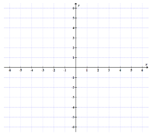
(d) Sketch a possible graph of $f(x)$ on the coordinate grid below.

05 - Special Limits and Continuity Learning Activity Image 1.png

Solution Key:

Part (a) — Horizontal Asymptotes: Examine end behavior as $x \to \pm\infty$ : $\lim_{x \to -\infty} f(x) = 5 \quad \text{and} \quad \lim_{x \to \infty} f(x) = 5$ Horizontal Asymptote Equation: $y = 5$
Part (b) — Vertical Asymptotes: Vertical asymptotes occur where limits blow up to $\pm\infty$ :
- At $x = -2$ : $\lim_{x \to -2^-} f(x) = -\infty$ and $\lim_{x \to -2^+} f(x) = \infty \implies x = -2$ .
- At $x = 3$ : $\lim_{x \to 3^-} f(x) = \infty$ and $\lim_{x \to 3^+} f(x) = -\infty \implies x = 3$ . Vertical Asymptote Equations: $x = -2 \quad \text{and} \quad x = 3$
Part (c) — Discontinuity Classification:
- At $x = 0$ : The two-sided limit exists ( $\lim_{x \to 0} f(x) = 3$ ), but $f(0)$ is undefined. This is a removable discontinuity (hole) at $(0, 3)$ .
- At $x = -2$ : The function approaches $\pm\infty$ . This is an infinite discontinuity.
- At $x = 3$ : The function approaches $\pm\infty$ . This is an infinite discontinuity.
Part (d) — Graphical Verification: The sketch must show:
- Approach to $y = 5$ as $x \to -\infty$ and $x \to +\infty$ .
- Vertical asymptote $x = -2$ with curve plunging to $-\infty$ from left and rising to $+\infty$ from right.
- Removable open circle at coordinate $(0, 3)$ with smooth curve passing through it.
- Vertical asymptote $x = 3$ with curve rising to $+\infty$ from left and plunging to $-\infty$ from right.

Show your steps and calculations here.

Regroup 3

Review how the three-part continuity rubric provides an unambiguous step-by-step diagnostic test for every boundary point.
Note how parameter-solving problems force Condition 3 ( $\lim_{x \to c} f(x) = f(c)$ ) to turn removable or jump points into seamless continuous transitions.

Synthesis Wrap-up

Core Takeaways from Session 05:
1. Composite limits are evaluated from the inside out; when inner limits approach $\pm\infty$ , evaluate the outer function's asymptotic behavior.
2. Trigonometric indeterminate forms $\frac{0}{0}$ resolve via the fundamental limit $\lim_{\theta \to 0} \frac{\sin\theta}{\theta} = 1$ and argument matching.
3. The Squeeze Theorem provides an analytical bridge for bounding high-frequency oscillatory systems between quadratic or linear envelopes.
4. Continuity requires the agreement of definition, limit existence, and value match ( $f(c) = \lim_{x \to c} f(x)$ ); failures cleanly partition into removable, jump, and infinite discontinuities.
Preview for Session 06: We will use the limiting process to define instantaneous rates of change and establish the formal limit definition of the derivative.
Homework Assignment: Complete Knewton Alta: Special Limits & Continuity.