MATH-181 (Calculus I) Curriculum

Session 02 - Introduction to Limits

Handout Worksheet
Fall Semester 2026
Session Objectives & Overview

By the end of this session, you will be able to:

  • Disentangle limit behavior from function values (the concept of approaching).
  • Diagnose and classify why a limit fails to exist (DNE).
  • Execute the limiting process to turn average rates into instantaneous rates.

Micro-Lecture

1. Introduction to Limits & Approaching Behavior

  • Mathematical Foundation: The study of limits bridges algebra and calculus by shifting focus from exact coordinates to infinitesimally close behavioral trends. We write lim⁡x→af(x)=L\lim_{x \to a} f(x) = Llimx→a​f(x)=L to denote that f(x)f(x)f(x) approaches LLL as xxx approaches aaa, but not equal to aaa.
  • Engineering Context: In real-world engineering, limits model fluid dynamics, particle physics near singularities, and aerodynamic transitions like supersonic shockwaves.

2. Limit Failures (DNE) & Discontinuities

  • Mathematical Foundation: According to the Existence Theorem for Two-Sided Limits, a two-sided limit exists if and only if both the left-hand and right-hand limits approach the same finite value. If they do not, or if the function grows without bound, or fluctuates infinitely, the limit does not exist (DNE).
  • Engineering Context: Classifying discontinuities (Jump, Infinite, and Removable) helps diagnose digital circuit signal instability, shockwave structures, and volatile systems.

3. Average vs. Instantaneous Rates

  • Mathematical Foundation: The average rate of change on [a,b][a, b][a,b] is the slope of the secant line f(b)−f(a)b−a\frac{f(b) - f(a)}{b - a}b−af(b)−f(a)​. The instantaneous rate of change is the limit of the average rates as the interval shrinks, which is the slope of the tangent line: lim⁡h→0f(x0+h)−f(x0)h\lim_{h \to 0} \frac{f(x_0 + h) - f(x_0)}{h}limh→0​hf(x0​+h)−f(x0​)​.
  • Engineering Context: Instantaneous rates drive real-time telemetry, sensor readings, and autonomous vehicle speed estimations.

Skill Block 1

Worked Example A: Numerical Evaluation (The Estimation Table)

Complete the table for f(x)=x2−9x−3f(x) = \frac{x^2 - 9}{x - 3}f(x)=x−3x2−9​ to find lim⁡x→3f(x)\lim_{x \to 3} f(x)limx→3​f(x).

Worked Solution:
  1. Left-Hand Trend (x→3−x \to 3^-x→3−): Plug values slightly less than 333 into the simplified path rule f(x)=x+3f(x) = x + 3f(x)=x+3:
    • f(2.9)=2.9+3=5.9f(2.9) = 2.9 + 3 = 5.9f(2.9)=2.9+3=5.9
    • f(2.99)=2.99+3=5.99f(2.99) = 2.99 + 3 = 5.99f(2.99)=2.99+3=5.99
    • f(2.999)=2.999+3=5.999f(2.999) = 2.999 + 3 = 5.999f(2.999)=2.999+3=5.999
  2. Right-Hand Trend (x→3+x \to 3^+x→3+): Plug values slightly greater than 333 into the path rule:
    • f(3.1)=3.1+3=6.1f(3.1) = 3.1 + 3 = 6.1f(3.1)=3.1+3=6.1
    • f(3.01)=3.01+3=6.01f(3.01) = 3.01 + 3 = 6.01f(3.01)=3.01+3=6.01
    • f(3.001)=3.001+3=6.001f(3.001) = 3.001 + 3 = 6.001f(3.001)=3.001+3=6.001
  3. Analyze Convergence: Assemble the table:
xxx approaches from left →\to→ 2.92.92.9 2.992.992.99 2.9992.9992.999 333 3.0013.0013.001 3.013.013.01 3.13.13.1 ←\leftarrow← xxx approaches from right
f(x)f(x)f(x) trend 5.95.95.9 5.995.995.99 5.9995.9995.999 ? 6.0016.0016.001 6.016.016.01 6.16.16.1

As xxx pinches closer to 333 from both sides, the output values head toward the distinct value 666. Therefore, the limit is:

lim⁡x→3x2−9x−3=6\lim_{x \to 3} \frac{x^2 - 9}{x - 3} = 6x→3lim​x−3x2−9​=6

Worked Example B: Graphical Evaluation (Holes vs. Solid Dots)

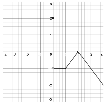
Use the piecewise graph provided below to evaluate the exact function value f(−1)f(-1)f(−1) and the limit value lim⁡x→−1f(x)\lim_{x \to -1} f(x)limx→−1​f(x).

02 - An Introduction to Limits Learning Activity Image 2.png
Worked Solution:
  1. Determine the Function Value f(−1)f(-1)f(−1): Look precisely along the vertical grid line x=−1x = -1x=−1. There is an open circle at a height of 222 and a solid dot at a height of 111. The solid dot represents the actual function value, so f(−1)=1f(-1) = 1f(−1)=1.
  2. Determine the Limit lim⁡x→−1f(x)\lim_{x \to -1} f(x)limx→−1​f(x): Trace along the lines of the graph as you approach x=−1x = -1x=−1 from both the left and right. Both paths lead directly to the open circle at height y=2y = 2y=2, so lim⁡x→−1f(x)=2\lim_{x \to -1} f(x) = 2limx→−1​f(x)=2.
  3. Compare Results: Note that lim⁡x→−1f(x)≠f(−1)\lim_{x \to -1} f(x) \neq f(-1)limx→−1​f(x)=f(−1) since 2≠12 \neq 12=1. This proves that a limit depends entirely on the expected trajectory of the path, independent of the actual point plotted at the destination.

Practice Problem 1: Concept & Reading Check

Open this Skill Block on the Memex to locate the information needed to answer the following:

  • (a) Under the Conceptual Framework section, what does the statement "limits look around the target, never at it" mean? How does it differ from algebra?
  • (b) According to Worked Example B, if the limit as x→−1x \to -1x→−1 is 222, why is the function value f(−1)f(-1)f(−1) equal to 111?
  • (c) Review the linked Engineering Application under the Engineering Applications section. How does limit behavior apply to electrical/computer engineering signal gain?
Solution Key:
  • (a) According to the Conceptual Framework section, algebra deals with exact coordinates at x=cx=cx=c, whereas limits describe the trend of outputs as we approach the input ccc from neighboring values.
  • (b) In Worked Example B, tracing the graph from both sides of x=−1x = -1x=−1 leads to the open circle at y=2y = 2y=2, which gives the limit. The solid dot at (−1,1)(-1, 1)(−1,1) represents the isolated function value, showing that path behavior (limit) can differ from the exact coordinate.
  • (c) As outlined in the Engineering Applications section under "Signal Cutoff Gain", limits allow electrical engineers to compute signal stability and gain near mathematical singularities (like division by zero at boundary cutoffs) by examining approaching trends.
Show your steps and calculations here.

Practice Problem 2

Complete the table given below for f(x)=x2−4x−2f(x) = \frac{x^2 - 4}{x - 2}f(x)=x−2x2−4​, then evaluate the given limits:

xxx 1.91.91.9 1.991.991.99 1.9991.9991.999 2.0012.0012.001 2.012.012.01 2.12.12.1
f(x)f(x)f(x)

(a) lim⁡x→2−x2−4x−2\lim_{x \to 2^-} \frac{x^2 - 4}{x - 2}limx→2−​x−2x2−4​ (b) lim⁡x→2+x2−4x−2\lim_{x \to 2^+} \frac{x^2 - 4}{x - 2}limx→2+​x−2x2−4​ (c) lim⁡x→2x2−4x−2\lim_{x \to 2} \frac{x^2 - 4}{x - 2}limx→2​x−2x2−4​ (d) Why can't we just find f(2)f(2)f(2) to determine lim⁡x→2f(x)\lim_{x \to 2} f(x)limx→2​f(x)?

Solution Key:
  1. Simplify the Function: Factor the numerator:
    f(x)=(x−2)(x+2)x−2=x+2(for x≠2)f(x) = \frac{(x-2)(x+2)}{x-2} = x+2 \quad (\text{for } x \neq 2)f(x)=x−2(x−2)(x+2)​=x+2(for x=2)
  2. Evaluate the Table:
    • f(1.9)=1.9+2=3.9f(1.9) = 1.9+2 = 3.9f(1.9)=1.9+2=3.9
    • f(1.99)=1.99+2=3.99f(1.99) = 1.99+2 = 3.99f(1.99)=1.99+2=3.99
    • f(1.999)=1.999+2=3.999f(1.999) = 1.999+2 = 3.999f(1.999)=1.999+2=3.999
    • f(2.001)=2.001+2=4.001f(2.001) = 2.001+2 = 4.001f(2.001)=2.001+2=4.001
    • f(2.01)=2.01+2=4.01f(2.01) = 2.01+2 = 4.01f(2.01)=2.01+2=4.01
    • f(2.1)=2.1+2=4.1f(2.1) = 2.1+2 = 4.1f(2.1)=2.1+2=4.1
  3. Evaluate the Limits:
    • (a) As x→2−x \to 2^-x→2−, f(x)f(x)f(x) approaches 444.
    • (b) As x→2+x \to 2^+x→2+, f(x)f(x)f(x) approaches 444.
    • (c) Since the left-hand and right-hand limits match, the two-sided limit exists and is equal to 444.
    • (d) Direct substitution of x=2x = 2x=2 gives f(2)=00f(2) = \frac{0}{0}f(2)=00​, which is undefined. The limit describes what height the function approaches as we get closer to x=2x=2x=2 from the sides, which is 444.
Show your steps and calculations here.

Practice Problem 3

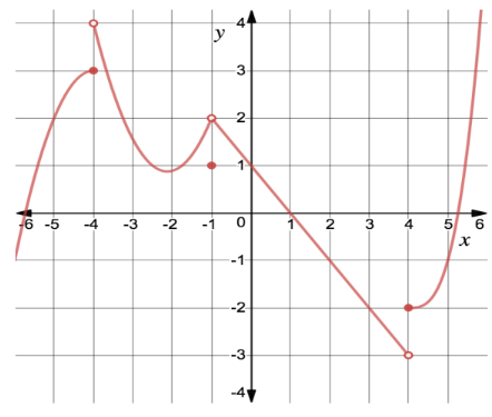
For the graph of f(x)f(x)f(x) given below, find the following values, if they exist. If it does not exist, state "DNE".

(a) f(−1)f(-1)f(−1) (d) lim⁡x→4+f(x)\lim_{x \to 4^+} f(x)limx→4+​f(x) (g) lim⁡x→−4−f(x)\lim_{x \to -4^-} f(x)limx→−4−​f(x)
(b) lim⁡x→−1f(x)\lim_{x \to -1} f(x)limx→−1​f(x) (e) lim⁡x→4−f(x)\lim_{x \to 4^-} f(x)limx→4−​f(x) (h) lim⁡x→−4f(x)\lim_{x \to -4} f(x)limx→−4​f(x)
(c) f(4)f(4)f(4) (f) lim⁡x→4f(x)\lim_{x \to 4} f(x)limx→4​f(x) (i) lim⁡x→−5f(x)\lim_{x \to -5} f(x)limx→−5​f(x)
02 - An Introduction to Limits Learning Activity Image 1.png
Solution Key:
  1. Part (a) - f(−1)f(-1)f(−1): At x=−1x = -1x=−1, there is an open circle at y=2y = 2y=2 and a solid dot at y=1y = 1y=1. The solid dot represents the function value, so f(−1)=1f(-1) = 1f(−1)=1.
  2. Part (b) - lim⁡x→−1f(x)\lim_{x \to -1} f(x)limx→−1​f(x): Approaching x=−1x = -1x=−1 from both sides, the curve targets the open circle at height y=2y = 2y=2. Thus, the limit is 222.
  3. Part (c) - f(4)f(4)f(4): Looking at x=4x = 4x=4, there is a solid dot at y=−2y = -2y=−2 and an open circle at y=−3y = -3y=−3. Therefore, f(4)=−2f(4) = -2f(4)=−2.
  4. Part (d) - lim⁡x→4+f(x)\lim_{x \to 4^+} f(x)limx→4+​f(x): Tracing the curve from the right toward x=4x = 4x=4, the curve approaches the solid dot at height y=−2y = -2y=−2.
  5. Part (e) - lim⁡x→4−f(x)\lim_{x \to 4^-} f(x)limx→4−​f(x): Tracing the line from the left toward x=4x = 4x=4, the line leads to the open circle at height y=−3y = -3y=−3.
  6. Part (f) - lim⁡x→4f(x)\lim_{x \to 4} f(x)limx→4​f(x): Since the left-hand limit (−3-3−3) and right-hand limit (−2-2−2) do not match, the two-sided limit does not exist (DNE\text{DNE}DNE).
  7. Part (g) - lim⁡x→−4−f(x)\lim_{x \to -4^-} f(x)limx→−4−​f(x): Tracing from the left toward x=−4x = -4x=−4, the curve ends at the solid dot at height y=3y = 3y=3.
  8. Part (h) - lim⁡x→−4f(x)\lim_{x \to -4} f(x)limx→−4​f(x): Tracing from the right toward x=−4x = -4x=−4, the curve approaches the open circle at y=4y = 4y=4. Since the left-hand limit (333) and right-hand limit (444) do not match, the two-sided limit is DNE\text{DNE}DNE.
  9. Part (i) - lim⁡x→−5f(x)\lim_{x \to -5} f(x)limx→−5​f(x): The curve is continuous and smooth at x=−5x = -5x=−5, passing exactly through height y=2y = 2y=2 from both directions, so the limit is 222.

Show your steps and calculations here.

Regroup 1

  • Discuss why a limit can exist at a hole where the function value is undefined or different.
  • Address the notation difference: f(a)f(a)f(a) represents the y-value at x=ax=ax=a, whereas lim⁡x→af(x)\lim_{x \to a} f(x)limx→a​f(x) represents the y-value approached by the path as xxx gets close to aaa.

Skill Block 2

Worked Example A: Analyzing a Jump Discontinuity

Analyze the function f(x)=∣x∣xf(x) = \frac{|x|}{x}f(x)=x∣x∣​ near x=0x = 0x=0 using the graph below to evaluate the one-sided limits and the two-sided limit.
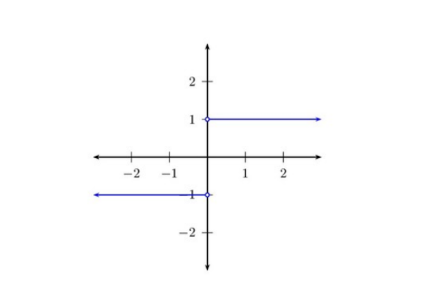
02 - Diagnosing and Classifying Why a Limit Fails to Exist (DNE) Image 1.png
Worked Solution:
  1. Evaluate Left-Hand Limit: Trace the graph from the left toward x=0x = 0x=0 (x<0x < 0x<0). The function forms a flat line at a height of −1-1−1:
    lim⁡x→0−∣x∣x=−1\lim_{x \to 0^-} \frac{|x|}{x} = -1x→0−lim​x∣x∣​=−1
  2. Evaluate Right-Hand Limit: Trace the graph from the right toward x=0x = 0x=0 (x>0x > 0x>0). The function forms a flat line at a height of 111:
    lim⁡x→0+∣x∣x=1\lim_{x \to 0^+} \frac{|x|}{x} = 1x→0+lim​x∣x∣​=1
  3. Determine Two-Sided Limit: Because the left-hand and right-hand limits do not match (−1≠1-1 \neq 1−1=1), by the Existence Theorem, the two-sided limit does not exist:
    lim⁡x→0∣x∣x=DNE\lim_{x \to 0} \frac{|x|}{x} = \text{DNE}x→0lim​x∣x∣​=DNE
    (Classification: Jump Discontinuity)

Worked Example B: Analyzing Unbounded Behavior

Evaluate lim⁡x→01x2\lim_{x \to 0} \frac{1}{x^2}limx→0​x21​ numerically and graphically.

02 - Diagnosing and Classifying Why a Limit Fails to Exist (DNE) Image 2.png
Worked Solution:
  1. Numerical Evaluation: Pick values that approach 000 from both sides:
    • f(±0.1)=1(0.1)2=100f(\pm 0.1) = \frac{1}{(0.1)^2} = 100f(±0.1)=(0.1)21​=100
    • f(±0.01)=1(0.01)2=10,000f(\pm 0.01) = \frac{1}{(0.01)^2} = 10,000f(±0.01)=(0.01)21​=10,000
    • f(±0.001)=1(0.001)2=1,000,000f(\pm 0.001) = \frac{1}{(0.001)^2} = 1,000,000f(±0.001)=(0.001)21​=1,000,000
  2. Analyze Trend: As inputs get closer to 000, the output values grow without bound toward positive infinity.
  3. Conclude: Graphically, both sides of the curve shoot straight up along the vertical asymptote x=0x = 0x=0. Since the values do not approach a single real number, the limit does not exist:
    lim⁡x→01x2=DNE(or +∞)(Reason: Unbounded Behavior)\lim_{x \to 0} \frac{1}{x^2} = \text{DNE} \quad (\text{or } +\infty) \quad \text{(Reason: Unbounded Behavior)}x→0lim​x21​=DNE(or +∞)(Reason: Unbounded Behavior)

Worked Example C: Analyzing Wildly Oscillating Behavior

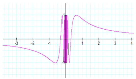
Determine why lim⁡x→0sin⁡(1x)\lim_{x \to 0} \sin\left(\frac{1}{x}\right)limx→0​sin(x1​) fails to exist using the tracking data.

Worked Solution:
  1. Analyze Data points as x→0+x \to 0^+x→0+:
    • At x=0.01  ⟹  f(x)=sin⁡(100)≈−0.5064x = 0.01 \implies f(x) = \sin(100) \approx -0.5064x=0.01⟹f(x)=sin(100)≈−0.5064
    • At x=0.001  ⟹  f(x)=sin⁡(1000)≈0.8269x = 0.001 \implies f(x) = \sin(1000) \approx 0.8269x=0.001⟹f(x)=sin(1000)≈0.8269
    • At x=0.0001  ⟹  f(x)=sin⁡(10000)≈−0.3056x = 0.0001 \implies f(x) = \sin(10000) \approx -0.3056x=0.0001⟹f(x)=sin(10000)≈−0.3056
    • At x=0.00001  ⟹  f(x)=sin⁡(100000)≈0.0357x = 0.00001 \implies f(x) = \sin(100000) \approx 0.0357x=0.00001⟹f(x)=sin(100000)≈0.0357
  2. Analyze Trend: As xxx approaches 000, the function value fluctuates rapidly and infinitely between −1-1−1 and 111. It never settles down or stabilizes near a single number.
  3. Conclude:
    lim⁡x→0sin⁡(1x)=DNE(Reason: Wildly Oscillating Behavior)\lim_{x \to 0} \sin\left(\frac{1}{x}\right) = \text{DNE} \quad \text{(Reason: Wildly Oscillating Behavior)}x→0lim​sin(x1​)=DNE(Reason: Wildly Oscillating Behavior)

Practice Problem 4: Concept & Reading Check

Open this Skill Block on the Memex to locate the information needed to answer the following:

  • (a) Under the Conceptual Framework section, list the three structural types of limit failures (DNE) covered in this block.
  • (b) Look at Worked Example A. Why does the two-sided limit lim⁡x→0∣x∣x\lim_{x \to 0} \frac{|x|}{x}limx→0​x∣x∣​ fail to exist? Detail the left-hand and right-hand values.
  • (c) In Worked Example C, why does the function values table show that lim⁡x→0sin⁡(1/x)\lim_{x \to 0} \sin(1/x)limx→0​sin(1/x) does not exist? What behavior does it exhibit?
Solution Key:
  • (a) The Conceptual Framework section lists three reasons a limit fails to exist:
    1. Jump Discontinuity: One-sided limits exist and are finite but differ.
    2. Unbounded Behavior: The function grows to positive or negative infinity (vertical asymptote).
    3. Wildly Oscillating Behavior: The function fluctuates endlessly between different values without converging.
  • (b) In Worked Example A, tracing the graph of f(x)=∣x∣xf(x) = \frac{|x|}{x}f(x)=x∣x∣​ near x=0x = 0x=0 yields a left-hand limit of −1-1−1 and a right-hand limit of 111. Since the left and right trajectories approach different values, the two-sided limit does not exist (a Jump Discontinuity).
  • (c) Tracing the data in Worked Example C shows that as x→0x \to 0x→0, the function values fluctuate back and forth between −1-1−1 and 111 (e.g. going from −0.5064→0.8269→−0.3056-0.5064 \to 0.8269 \to -0.3056−0.5064→0.8269→−0.3056). The function never stabilizes or converges to a single coordinate, which is classified as Wildly Oscillating Behavior.
Show your steps and calculations here.

Practice Problem 5

Evaluate the limit analytically or graphically. If the limit does not exist, classify the failure using one of the three structural behaviors (Jump Discontinuity, Unbounded Behavior, or Wildly Oscillating Behavior):

lim⁡x→3f(x),where f(x)={2x−1:x<310−x:x≥3\lim_{x \to 3} f(x), \quad \text{where } f(x) = \begin{cases} 2x - 1 & : x < 3 \\ 10 - x & : x \ge 3 \end{cases}x→3lim​f(x),where f(x)={2x−110−x​:x<3:x≥3​

Solution Key:
  • Left-hand limit: lim⁡x→3−f(x)=lim⁡x→3−(2x−1)=2(3)−1=5\lim_{x \to 3^-} f(x) = \lim_{x \to 3^-} (2x - 1) = 2(3) - 1 = 5limx→3−​f(x)=limx→3−​(2x−1)=2(3)−1=5
  • Right-hand limit: lim⁡x→3+f(x)=lim⁡x→3+(10−x)=10−3=7\lim_{x \to 3^+} f(x) = \lim_{x \to 3^+} (10 - x) = 10 - 3 = 7limx→3+​f(x)=limx→3+​(10−x)=10−3=7
  • Since 5≠75 \neq 75=7, the two-sided limit fails to exist. Because both one-sided limits are finite numbers that do not match, this failure is classified as a Jump Discontinuity.
Show your steps and calculations here.

Practice Problem 6

Evaluate the limit analytically. If the limit does not exist, classify the failure using one of the three structural behaviors (Jump Discontinuity, Unbounded Behavior, or Wildly Oscillating Behavior):

lim⁡x→23x−2\lim_{x \to 2} \frac{3}{x - 2}x→2lim​x−23​

Solution Key:
  • As x→2−x \to 2^-x→2−, the denominator x−2x - 2x−2 is negative and approaches 000, so 3x−2→−∞\frac{3}{x - 2} \to -\inftyx−23​→−∞.
  • As x→2+x \to 2^+x→2+, the denominator x−2x - 2x−2 is positive and approaches 000, so 3x−2→+∞\frac{3}{x - 2} \to +\inftyx−23​→+∞.
  • Because the function values grow infinitely large (in absolute value) and do not approach a finite real number as x→2x \to 2x→2, the limit is DNE\text{DNE}DNE due to Unbounded Behavior (a vertical asymptote at x=2x = 2x=2).
Show your steps and calculations here.

Practice Problem 7

Evaluate the limit analytically. If the limit does not exist, classify the failure using one of the three structural behaviors (Jump Discontinuity, Unbounded Behavior, or Wildly Oscillating Behavior):

lim⁡x→0+cos⁡(πx)\lim_{x \to 0^+} \cos\left(\frac{\pi}{x}\right)x→0+lim​cos(xπ​)

Solution Key:
  • As x→0+x \to 0^+x→0+, the angle θ=πx\theta = \frac{\pi}{x}θ=xπ​ approaches +∞+\infty+∞.
  • The cosine function cos⁡(θ)\cos(\theta)cos(θ) oscillates continuously between −1-1−1 and 111. As xxx gets closer to 000, these oscillations happen infinitely fast. For example:
    • x=1  ⟹  cos⁡(π)=−1x = 1 \implies \cos(\pi) = -1x=1⟹cos(π)=−1
    • x=0.5  ⟹  cos⁡(2π)=1x = 0.5 \implies \cos(2\pi) = 1x=0.5⟹cos(2π)=1
    • x=0.25  ⟹  cos⁡(4π)=1x = 0.25 \implies \cos(4\pi) = 1x=0.25⟹cos(4π)=1
    • x=2/3  ⟹  cos⁡(1.5π)=0x = 2/3 \implies \cos(1.5\pi) = 0x=2/3⟹cos(1.5π)=0
  • The function values do not stabilize or settle near any single number. Thus, the limit is DNE\text{DNE}DNE due to Wildly Oscillating Behavior.

Show your steps and calculations here.

Regroup 2

  • Discuss how physical systems exhibit these failures: a switch flipping represents a jump discontinuity; a capacitor charging rate near a singularity can model unbounded behavior; and noise/chatter in a signal can model oscillating behavior.

Skill Block 3

Worked Example A: Calculating Average Rate of Change

Find the average rate of change of f(x)=sin⁡(x)f(x) = \sin(x)f(x)=sin(x) over the interval [0,π6]\left[0, \frac{\pi}{6}\right][0,6π​].

Worked Solution:
  1. Evaluate Function at Endpoints:
    • f(0)=sin⁡(0)=0f(0) = \sin(0) = 0f(0)=sin(0)=0
    • f(π6)=sin⁡(π6)=0.5=12f\left(\frac{\pi}{6}\right) = \sin\left(\frac{\pi}{6}\right) = 0.5 = \frac{1}{2}f(6π​)=sin(6π​)=0.5=21​
  2. Apply Formula:
    Average Rate=f(π/6)−f(0)π/6−0=0.5−0π/6=0.5π/6=3π≈0.9549\text{Average Rate} = \frac{f(\pi/6) - f(0)}{\pi/6 - 0} = \frac{0.5 - 0}{\pi/6} = \frac{0.5}{\pi/6} = \frac{3}{\pi} \approx 0.9549Average Rate=π/6−0f(π/6)−f(0)​=π/60.5−0​=π/60.5​=π3​≈0.9549
    The average rate of change is 3π≈0.9549\frac{3}{\pi} \approx 0.9549π3​≈0.9549.

Worked Example B: The Shifting Interval Process (Kinematics)

A rock is launched vertically upward from the ground with an initial speed of 85 ft/sec85\text{ ft/sec}85 ft/sec. Its position equation is modeled by s(t)=−16t2+85ts(t) = -16t^2 + 85ts(t)=−16t2+85t. Use a sequence of shrinking intervals to estimate the instantaneous velocity of the rock at exactly t=1t = 1t=1 second.

Worked Solution:
  1. Find s(1)s(1)s(1):
    s(1)=−16(1)2+85(1)=69 fts(1) = -16(1)^2 + 85(1) = 69\text{ ft}s(1)=−16(1)2+85(1)=69 ft
  2. Calculate Average Velocity over broad interval [1,2][1, 2][1,2]:
    • s(2)=−16(2)2+85(2)=106 fts(2) = -16(2)^2 + 85(2) = 106\text{ ft}s(2)=−16(2)2+85(2)=106 ft
    • Average Velocity=s(2)−s(1)2−1=106−691=37 ft/sec\text{Average Velocity} = \frac{s(2) - s(1)}{2 - 1} = \frac{106 - 69}{1} = 37\text{ ft/sec}Average Velocity=2−1s(2)−s(1)​=1106−69​=37 ft/sec
  3. Shrink interval to [1,1.1][1, 1.1][1,1.1]:
    • s(1.1)=−16(1.1)2+85(1.1)=74.14 fts(1.1) = -16(1.1)^2 + 85(1.1) = 74.14\text{ ft}s(1.1)=−16(1.1)2+85(1.1)=74.14 ft
    • Average Velocity=74.14−691.1−1=5.140.1=51.4 ft/sec\text{Average Velocity} = \frac{74.14 - 69}{1.1 - 1} = \frac{5.14}{0.1} = 51.4\text{ ft/sec}Average Velocity=1.1−174.14−69​=0.15.14​=51.4 ft/sec
  4. Shrink interval to [1,1.01][1, 1.01][1,1.01]:
    • s(1.01)=−16(1.01)2+85(1.01)=69.5284 fts(1.01) = -16(1.01)^2 + 85(1.01) = 69.5284\text{ ft}s(1.01)=−16(1.01)2+85(1.01)=69.5284 ft
    • Average Velocity=69.5284−691.01−1=0.52840.01=52.84 ft/sec\text{Average Velocity} = \frac{69.5284 - 69}{1.01 - 1} = \frac{0.5284}{0.01} = 52.84\text{ ft/sec}Average Velocity=1.01−169.5284−69​=0.010.5284​=52.84 ft/sec
  5. Shrink interval to [1,1.001][1, 1.001][1,1.001]:
    • s(1.001)=−16(1.001)2+85(1.001)=69.052984 fts(1.001) = -16(1.001)^2 + 85(1.001) = 69.052984\text{ ft}s(1.001)=−16(1.001)2+85(1.001)=69.052984 ft
    • Average Velocity=69.052984−691.001−1=0.0529840.001=52.984 ft/sec\text{Average Velocity} = \frac{69.052984 - 69}{1.001 - 1} = \frac{0.052984}{0.001} = 52.984\text{ ft/sec}Average Velocity=1.001−169.052984−69​=0.0010.052984​=52.984 ft/sec
  6. Infer the Limit: As the time interval length approaches 000, the average velocities (37→51.4→52.84→52.98437 \to 51.4 \to 52.84 \to 52.98437→51.4→52.84→52.984) converge toward 53 ft/sec53\text{ ft/sec}53 ft/sec. This is the estimated instantaneous velocity at t=1t = 1t=1.

Practice Problem 8: Concept & Reading Check

Open this Skill Block on the Memex to locate the information needed to answer the following:

  • (a) Under the Conceptual Framework section, what geometric slopes do the secant line and tangent line represent?
  • (b) Explain why we cannot compute the instantaneous rate of change by simply setting the interval length h=0h = 0h=0 in the formula. What mathematical form does it produce?
  • (c) Trace Worked Example B. What sequence of average velocities was calculated, and what value did they converge to?
Solution Key:
  • (a) According to the Conceptual Framework section, the average rate of change corresponds to the slope of a secant line between two distinct points. The instantaneous rate of change corresponds to the slope of a tangent line at a single point.
  • (b) As explained in the Conceptual Framework, substituting h=0h = 0h=0 directly into the rate expression yields f(x0)−f(x0)0=00\frac{f(x_0) - f(x_0)}{0} = \frac{0}{0}0f(x0​)−f(x0​)​=00​, which is undefined. We must use the limiting process (h→0h \to 0h→0) to evaluate the approaching behavior.
  • (c) Tracing the solution in Worked Example B, the sequence of average velocities calculated over shrinking intervals is:
    • [1,2]  ⟹  37 ft/sec[1, 2] \implies 37\text{ ft/sec}[1,2]⟹37 ft/sec
    • [1,1.1]  ⟹  51.4 ft/sec[1, 1.1] \implies 51.4\text{ ft/sec}[1,1.1]⟹51.4 ft/sec
    • [1,1.01]  ⟹  52.84 ft/sec[1, 1.01] \implies 52.84\text{ ft/sec}[1,1.01]⟹52.84 ft/sec
    • [1,1.001]  ⟹  52.984 ft/sec[1, 1.001] \implies 52.984\text{ ft/sec}[1,1.001]⟹52.984 ft/sec These values converge to 53 ft/sec53\text{ ft/sec}53 ft/sec as the time interval approaches 0.
Show your steps and calculations here.

Practice Problem 9

Find the average rate of change of the polynomial function over the given interval:

f(x)=3x2−3x+5on [−1,2]f(x) = 3x^2 - 3x + 5 \quad \text{on } [-1, 2]f(x)=3x2−3x+5on [−1,2]

Solution Key:
  1. Evaluate at x=2x = 2x=2:
    f(2)=3(2)2−3(2)+5=12−6+5=11f(2) = 3(2)^2 - 3(2) + 5 = 12 - 6 + 5 = 11f(2)=3(2)2−3(2)+5=12−6+5=11
  2. Evaluate at x=−1x = -1x=−1:
    f(−1)=3(−1)2−3(−1)+5=3+3+5=11f(-1) = 3(-1)^2 - 3(-1) + 5 = 3 + 3 + 5 = 11f(−1)=3(−1)2−3(−1)+5=3+3+5=11
  3. Compute the average rate of change:
    Average Rate=f(2)−f(−1)2−(−1)=11−113=0\text{Average Rate} = \frac{f(2) - f(-1)}{2 - (-1)} = \frac{11 - 11}{3} = 0Average Rate=2−(−1)f(2)−f(−1)​=311−11​=0
Show your steps and calculations here.

Practice Problem 10

Find the average rate of change of the trigonometric function over the given interval:

g(t)=3cos⁡2(t)on [0,π6]g(t) = 3\cos^2(t) \quad \text{on } \left[0, \frac{\pi}{6}\right]g(t)=3cos2(t)on [0,6π​]

Solution Key:
  1. Evaluate at t=π6t = \frac{\pi}{6}t=6π​:
    g(π6)=3[cos⁡(π6)]2=3(32)2=3(34)=94g\left(\frac{\pi}{6}\right) = 3\left[\cos\left(\frac{\pi}{6}\right)\right]^2 = 3\left(\frac{\sqrt{3}}{2}\right)^2 = 3\left(\frac{3}{4}\right) = \frac{9}{4}g(6π​)=3[cos(6π​)]2=3(23​​)2=3(43​)=49​
  2. Evaluate at t=0t = 0t=0:
    g(0)=3[cos⁡(0)]2=3(1)2=3g(0) = 3[\cos(0)]^2 = 3(1)^2 = 3g(0)=3[cos(0)]2=3(1)2=3
  3. Compute the average rate of change:
    Average Rate=g(π/6)−g(0)π/6−0=94−3π6=−34π6=−34⋅6π=−184π=−92π≈−1.4324\text{Average Rate} = \frac{g(\pi/6) - g(0)}{\pi/6 - 0} = \frac{\frac{9}{4} - 3}{\frac{\pi}{6}} = \frac{-\frac{3}{4}}{\frac{\pi}{6}} = -\frac{3}{4} \cdot \frac{6}{\pi} = -\frac{18}{4\pi} = -\frac{9}{2\pi} \approx -1.4324Average Rate=π/6−0g(π/6)−g(0)​=6π​49​−3​=6π​−43​​=−43​⋅π6​=−4π18​=−2π9​≈−1.4324
Show your steps and calculations here.

Practice Problem 11

If a rock is thrown upward on the planet Mars with a velocity of 20 m/s20\text{ m/s}20 m/s, its height in meters ttt seconds later is given by s(t)=20t−2t2s(t) = 20t - 2t^2s(t)=20t−2t2.

(a) Find the average velocity of the rock over the given time intervals:

  • i. [1,1.1][1, 1.1][1,1.1]
  • ii. [1,1.01][1, 1.01][1,1.01]
  • iii. [1,1.001][1, 1.001][1,1.001]
  • iv. [1,1.0001][1, 1.0001][1,1.0001] (b) Estimate the instantaneous velocity when t=1t = 1t=1.
Solution Key:
  1. Find Initial Value:
    s(1)=20(1)−2(1)2=18 ms(1) = 20(1) - 2(1)^2 = 18\text{ m}s(1)=20(1)−2(1)2=18 m
  2. Compute Average Velocities:
    • i. Interval [1,1.1][1, 1.1][1,1.1]:
      • s(1.1)=20(1.1)−2(1.21)=22−2.42=19.58 ms(1.1) = 20(1.1) - 2(1.21) = 22 - 2.42 = 19.58\text{ m}s(1.1)=20(1.1)−2(1.21)=22−2.42=19.58 m
      • Average Velocity=19.58−181.1−1=1.580.1=15.8 m/s\text{Average Velocity} = \frac{19.58 - 18}{1.1 - 1} = \frac{1.58}{0.1} = 15.8\text{ m/s}Average Velocity=1.1−119.58−18​=0.11.58​=15.8 m/s
    • ii. Interval [1,1.01][1, 1.01][1,1.01]:
      • s(1.01)=20(1.01)−2(1.01)2=20.2−2.0402=18.1598 ms(1.01) = 20(1.01) - 2(1.01)^2 = 20.2 - 2.0402 = 18.1598\text{ m}s(1.01)=20(1.01)−2(1.01)2=20.2−2.0402=18.1598 m
      • Average Velocity=18.1598−181.01−1=0.15980.01=15.98 m/s\text{Average Velocity} = \frac{18.1598 - 18}{1.01 - 1} = \frac{0.1598}{0.01} = 15.98\text{ m/s}Average Velocity=1.01−118.1598−18​=0.010.1598​=15.98 m/s
    • iii. Interval [1,1.001][1, 1.001][1,1.001]:
      • s(1.001)=20(1.001)−2(1.001)2=20.02−2.004002=18.015998 ms(1.001) = 20(1.001) - 2(1.001)^2 = 20.02 - 2.004002 = 18.015998\text{ m}s(1.001)=20(1.001)−2(1.001)2=20.02−2.004002=18.015998 m
      • Average Velocity=18.015998−181.001−1=0.0159980.001=15.998 m/s\text{Average Velocity} = \frac{18.015998 - 18}{1.001 - 1} = \frac{0.015998}{0.001} = 15.998\text{ m/s}Average Velocity=1.001−118.015998−18​=0.0010.015998​=15.998 m/s
    • iv. Interval [1,1.0001][1, 1.0001][1,1.0001]:
      • s(1.0001)=20(1.0001)−2(1.0001)2=20.002−2.00040002=18.00159998 ms(1.0001) = 20(1.0001) - 2(1.0001)^2 = 20.002 - 2.00040002 = 18.00159998\text{ m}s(1.0001)=20(1.0001)−2(1.0001)2=20.002−2.00040002=18.00159998 m
      • Average Velocity=18.00159998−181.0001−1=0.001599980.0001=15.9998 m/s\text{Average Velocity} = \frac{18.00159998 - 18}{1.0001 - 1} = \frac{0.00159998}{0.0001} = 15.9998\text{ m/s}Average Velocity=1.0001−118.00159998−18​=0.00010.00159998​=15.9998 m/s
  3. Estimate Instantaneous Velocity: Looking at the sequence of average velocities:
    15.8→15.98→15.998→15.999815.8 \to 15.98 \to 15.998 \to 15.999815.8→15.98→15.998→15.9998
    As the time interval length approaches zero, the values converge to 16 m/s16\text{ m/s}16 m/s.

Show your steps and calculations here.

Regroup 3

  • Discuss how a physical instantaneous velocity can be measured (such as radar speedometer approximating by taking very short time intervals).

Synthesis Wrap-up

  • Core takeaways from Session 02:
    1. Limits describe paths, functions describe coordinates. They do not have to match.
    2. Limits DNE when directional paths disagree (Jump), shoot to infinity (Asymptote), or fluctuate endlessly (Oscillation).
    3. Average rates (secant line slopes) over shrinking intervals converge to the instantaneous rate (tangent line slope) via a limiting process.
  • Connections to Knewton Alta Homework: Introduction to Limits.